Introductory Sage Tutorial

This Sage document is the first in a series of tutorials developed for the MAA PREP Workshop “Sage: Using Open-Source Mathematics Software with Undergraduates” (funding provided by NSF DUE 0817071). It is licensed under the Creative Commons Attribution-ShareAlike 3.0 license (CC BY-SA).

If you are unsure how to log on to a Sage server, start using a local installation, or to create a new worksheet, you might find the prelude on logging in helpful.

Otherwise, you can continue with this tutorial, which has the following sections:

• Evaluating Sage Commands

  • See Evaluating in the Jupyter notebook for the Jupyter notebook

• Functions in Sage

• Help inside Sage

• Annotating with Sage

  • See Jupyter Annotation for the Jupyter notebook

This tutorial only introduces the most basic level of functionality. Later tutorials address topics such as calculus, advanced plotting, and a wide variety of specific mathematical topics.

Evaluating Sage Commands

Or, How do I get Sage to do some math?

• See Evaluating in the Jupyter notebook for the Jupyter notebook

Evaluating in the Jupyter notebook

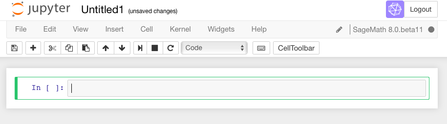
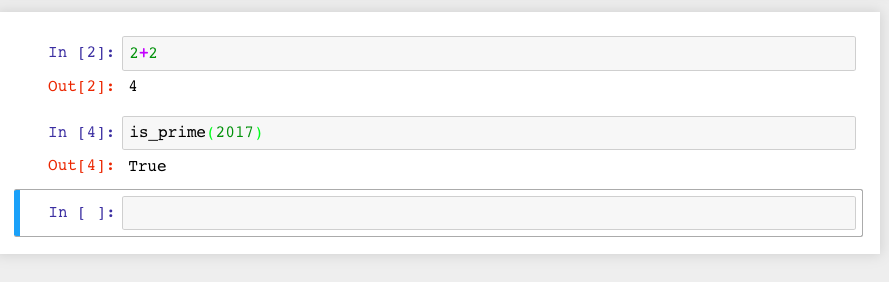
In a Jupyter worksheet, there are little boxes called input cells or code cells. They should be about the width of your browser.

To do math in a Jupyter cell, one must do two things.

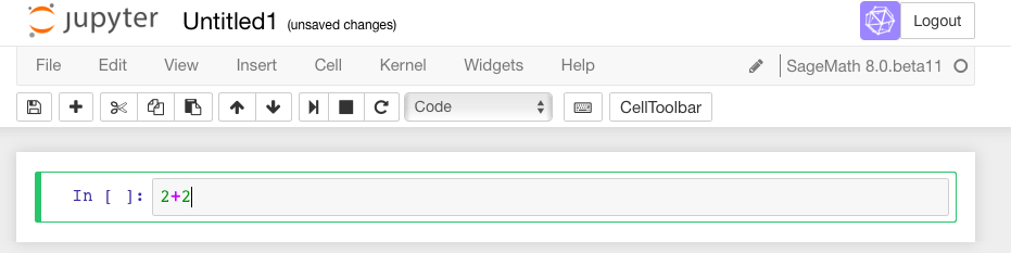
• First, click inside the cell so that the cell is active (i.e., has a bright green border). This was already the case in the first cell above. (If it is blue, the Jupyter notebook is in “command mode”). Type some math in it.

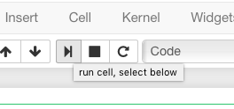
• Then, there are two options. A not-very-evident icon that looks like the “play” symbol on a recording device can be clicked:

  

  Or one can use the keyboard shortcut of holding down the Shift key while you press the Enter key. We call this Shift + Enter.

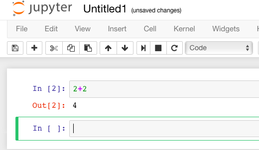
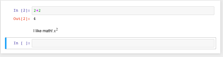
Sage prints out its response just below the cell (that’s the 4 below, so Sage confirms that \(2+2=4\)). Note also that Sage has automatically made a new cell, and made it active, after you evaluated your first cell.

To do more mathematics, just do the same thing with more cells!

One has to learn a variety of keyboard shortcuts or click on various menu items to manipulate cells. There is a help menu to get you started on this; the Jupyter developers also maintain an example notebook which may assist you.

Functions in Sage

To start out, let’s explore how to define and use functions in Sage.

For a typical mathematical function, it’s pretty straightforward to define it. Below, we define a function.

\[f(x)=x^2\]

Sage

sage: f(x)=x^2

Python

>>> from sage.all import *
>>> __tmp__=var("x"); f = symbolic_expression(x**Integer(2)).function(x)

Since all we wanted was to create the function \(f(x)\), Sage just does this and doesn’t print anything out back to us.

We can check the definition by asking Sage what f(x) is:

Sage

sage: f(x)
x^2

Python

>>> from sage.all import *
>>> f(x)
x^2

If we just ask Sage what f is (as opposed to f(x)), Sage prints out the standard mathematical notation for a function that maps a variable \(x\) to the value \(x^2\) (with the “maps to” arrow \(\mapsto\) as |-->).

Sage

sage: f
x |--> x^2

Python

>>> from sage.all import *
>>> f
x |--> x^2

We can evaluate \(f\) at various values.

Sage

sage: f(3)
9

Python

>>> from sage.all import *
>>> f(Integer(3))
9

Sage

sage: f(3.1)
9.61000000000000

Python

>>> from sage.all import *
>>> f(RealNumber('3.1'))
9.61000000000000

Sage

sage: f(31/10)
961/100

Python

>>> from sage.all import *
>>> f(Integer(31)/Integer(10))
961/100

Notice that the output type changes depending on whether the input had a decimal; we’ll see that again below.

Naturally, we are not restricted to \(x\) as a variable. In the next cell, we define the function \(g(y)=2y-1\).

Sage

sage: g(y)=2*y-1

Python

>>> from sage.all import *
>>> __tmp__=var("y"); g = symbolic_expression(Integer(2)*y-Integer(1)).function(y)

However, we need to make sure we do define a function if we use a new variable. In the next cell, we see what happens if we try to use a random input by itself.

Sage

sage: z^2
Traceback (most recent call last):
...
NameError: name 'z' is not defined

Python

>>> from sage.all import *
>>> z**Integer(2)
Traceback (most recent call last):
...
NameError: name 'z' is not defined

This is explained in some detail in following tutorials. At this point, it suffices to know using the function notation (like g(y)) tells Sage you are serious about y being a variable.

One can also do this with the var('z') notation below.

Sage

sage: var('z')
z
sage: z^2
z^2

Python

>>> from sage.all import *
>>> var('z')
z
>>> z**Integer(2)
z^2

This also demonstrates that we can put several commands in one cell, each on a separate line. The output of the last command (if any) is printed as the output of the cell.

Sage knows various common mathematical constants, like \(\pi\) (pi) and \(e\).

Sage

sage: f(pi)
pi^2

Python

>>> from sage.all import *
>>> f(pi)
pi^2

Sage

sage: f(e^-1)
e^(-2)

Python

>>> from sage.all import *
>>> f(e**-Integer(1))
e^(-2)

In order to see a numeric approximation for an expression, just type the expression inside the parentheses of N().

Sage

sage: N(f(pi))
9.86960440108936

Python

>>> from sage.all import *
>>> N(f(pi))
9.86960440108936

Another option, often more useful in practice, is having the expression immediately followed by .n() (note the dot).

Sage

sage: f(pi).n()
9.86960440108936

Python

>>> from sage.all import *
>>> f(pi).n()
9.86960440108936

For now, we won’t go in great depth explaining the reasons behind this syntax, which may be new to you. For those who are interested, Sage often uses this type of syntax (known as “object-oriented”) because…

• Sage uses the Python programming language, which uses this syntax, ‘under the hood’, and

• Because it makes it easier to distinguish among

• The mathematical object,

• The thing you are doing to it, and

• Any ancillary arguments.

For example, the following numerically evaluates (n) the constant \(\pi\) (pi) to twenty digits (digits=20).

Sage

sage: pi.n(digits=20)
3.1415926535897932385

Python

>>> from sage.all import *
>>> pi.n(digits=Integer(20))
3.1415926535897932385

Sage has lots of common mathematical functions built in, like \(\sqrt{x}\) (sqrt(x)) and \(\ln(x)\) (ln(x) or log(x)).

Sage

sage: log(3)
log(3)

Python

>>> from sage.all import *
>>> log(Integer(3))
log(3)

Notice that there is no reason to numerically evaluate \(\log(3)\), so Sage keeps it symbolic. The same is true in the next cell - \(2\log(3)=\log(9)\), but there isn’t any reason to do that; after all, depending on what you want, \(\log(9)\) may be simpler or less simple than you need.

Sage

sage: log(3)+log(3)
2*log(3)

Python

>>> from sage.all import *
>>> log(Integer(3))+log(Integer(3))
2*log(3)

Sage

sage: log(3).n()
1.09861228866811

Python

>>> from sage.all import *
>>> log(Integer(3)).n()
1.09861228866811

Notice again that Sage tries to respect the type of input as much as possible; adding the decimal tells Sage that we have approximate input and want a more approximate answer. (Full details are a little too complicated for this introduction.)

Sage

sage: log(3.)
1.09861228866811

Python

>>> from sage.all import *
>>> log(RealNumber('3.'))
1.09861228866811

Sage

sage: sqrt(2)
sqrt(2)

Python

>>> from sage.all import *
>>> sqrt(Integer(2))
sqrt(2)

If we want this to look nicer, we can use the show command. We’ll see more of this sort of thing below.

Sage

sage: show(sqrt(2))

Python

>>> from sage.all import *
>>> show(sqrt(Integer(2)))

\[\sqrt{2}\]

Sage

sage: sqrt(2).n()
1.41421356237310

Python

>>> from sage.all import *
>>> sqrt(Integer(2)).n()
1.41421356237310

Do you remember what \(f\) does?

Sage

sage: f(sqrt(2))
2

Python

>>> from sage.all import *
>>> f(sqrt(Integer(2)))
2

We can also plot functions easily.

Sage

sage: plot(f, (x,-3,3))
Graphics object consisting of 1 graphics primitive

Python

>>> from sage.all import *
>>> plot(f, (x,-Integer(3),Integer(3)))
Graphics object consisting of 1 graphics primitive

In another tutorial, we will go more in depth with plotting. Here, note that the preferred syntax has the variable and endpoints for the plotting domain in parentheses, separated by commas.

If you are feeling bold, plot the sqrt function in the next cell between 0 and 100.

Help inside Sage

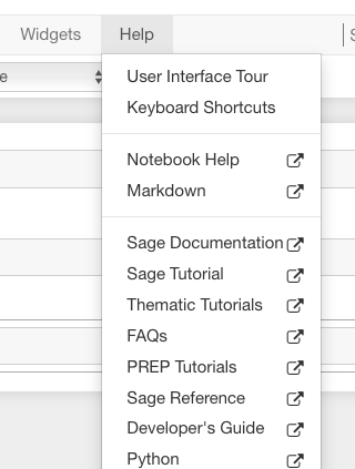
There are various ways to get help for doing things in Sage. Here are several common ways to get help as you are working in a Sage worksheet.

Documentation

Sage includes extensive documentation covering thousands of functions, with many examples, tutorials, and other helps.

• One way to access these is to click the “Help” link at the top right of any worksheet, then click your preferred option at the top of the help page.

• They are also available any time online at the Sage website, which has many other links, like video introductions.

• The Quick Reference cards are another useful tool once you get more familiar with Sage.

Our main focus in this tutorial, though, is help you can immediately access from within a worksheet, where you don’t have to do any of those things.

Tab completion

The most useful help available in the notebook is “tab completion”. The idea is that even if you aren’t one hundred percent sure of the name of a command, the first few letters should still be enough to help find it. Here’s an example.

• Suppose you want to do a specific type of plot - maybe a slope field plot - but aren’t quite sure what will do it.

• Still, it seems reasonable that the command might start with pl.

• Then one can type pl in an input cell, and then press the Tab key to see all the commands that start with the letters pl.

Try tabbing after the pl in the following cell to see all the commands that start with the letters pl. You should see that plot_slope_field is one of them.

Sage

sage: pl

Python

>>> from sage.all import *
>>> pl

To pick one, just click on it; to stop viewing them, press the Escape key.

You can also use this to see what you can do to an expression or mathematical object.

• Assuming your expression has a name, type it;

• Then type a period after it,

• Then press tab.

You will see a list pop up of all the things you can do to the expression.

To try this, evaluate the following cell, just to make sure \(f\) is defined.

Sage

sage: f(x)=x^2

Python

>>> from sage.all import *
>>> __tmp__=var("x"); f = symbolic_expression(x**Integer(2)).function(x)

Now put your cursor after the period and press your Tab key.

Sage

sage: f.

Python

>>> from sage.all import *
>>> f.

Again, Escape should remove the list.

One of the things in that list above was integrate. Let’s try it.

Sage

sage: f.integrate(x)
x |--> 1/3*x^3

Python

>>> from sage.all import *
>>> f.integrate(x)
x |--> 1/3*x^3

Finding documentation

Or, Why all the question marks?

In the previous example, you might have wondered why I needed to put f.integrate(x) rather than just f.integrate(), by analogy with sqrt(2).n().

To find out, there is another help tool one can use from right inside the notebook. Almost all documentation in Sage has extensive examples that can illustrate how to use the function.

• As with tab completion, type the expression, period, and the name of the function.

• Then type a question mark.

• Press tab or evaluate to see the documentation.

To see how this help works, move your cursor after the question mark below and press Tab.

Sage

sage: f.integrate?

Python

>>> from sage.all import *
>>> f.integrate?

The examples illustrate that the syntax requires f.integrate(x) and not just f.integrate(). (After all, the latter could be ambiguous if several variables had already been defined).

To stop viewing the documentation after pressing Tab, you can press the Escape key, just like with the completion of options.

If you would like the documentation to be visible longer-term, you can evaluate a command with the question mark (like below) to access the documentation, rather than just tabbing. Then it will stay there until you remove the input cell.

Sage

sage: binomial?

Python

>>> from sage.all import *
>>> binomial?

Try this with another function!

Finding the source

There is one more source of help you may find useful in the long run, though perhaps not immediately.

• One can use two question marks after a function name to pull up the documentation and the source code for the function.

• Again, to see this help, you can either evaluate a cell like below, or just move your cursor after the question mark and press tab.

The ability to see the code (the underlying instructions to the computer) is one of Sage’s great strengths. You can see all the code to everything .

This means:

• You can see what Sage is doing.

• Your curious students can see what is going on.

• And if you find a better way to do something, then you can see how to change it!

Sage

sage: binomial??

Python

>>> from sage.all import *
>>> binomial??

Annotating with Sage

Whether one uses Sage in the classroom or in research, it is usually helpful to describe to the reader what is being done, such as in the description you are now reading.

• Jupyter Annotation

Jupyter Annotation

Thanks to a styling language called Markdown and the TeX rendering engine called MathJax, you can type much more in Sage than just Sage commands. This math-aware setup makes Sage perfect for annotating computations.

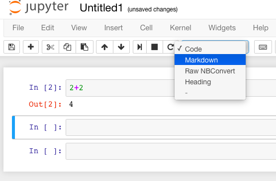
Jupyter notebook can function as a word processor. To use this functionality, we create a Markdown cell (as opposed to a input cell that contains Sage commands that Sage evaluates).

To do this without the keyboard shortcut, there is a menu for each cell; select “Markdown”.

Now you can type in whatever you want, including mathematics using LaTeX.

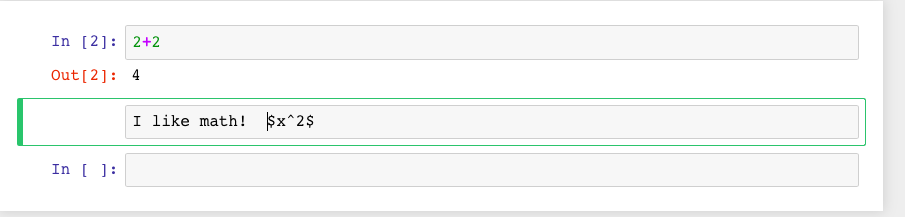
Then evaluate the cell (for instance, with “Shift-Enter”):

Markdown supports a fair amount of basic formatting, such as bold, underline, basic lists, and so forth.

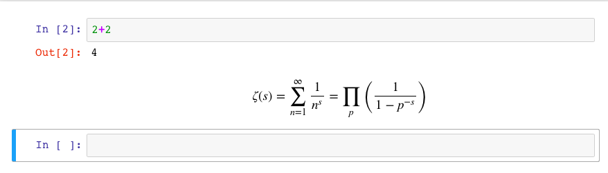
It can be fun to type in fairly complicated math, like this:

\[\zeta(s)=\sum_{n=1}^{\infty}\frac{1}{n^s}=\prod_p \left(\frac{1}{1-p^{-s}}\right)\; .\]

One just types things like:

$$\zeta(s)=\sum_{n=1}^{\infty}\frac{1}{n^s}=\prod_p \left(\frac{1}{1-p^{-s}}\right)$$

in a Markdown cell.

Of course, one can do much more, since Sage can execute arbitrary commands in the Python programming language, as well as output nicely formatted HTML, and so on. If you have enough programming experience to do things like this, go for it!

Sage

sage: html("Sage is <a style='text-decoration:line-through'>somewhat</a> <b>really</b> cool! <p style='color:red'>(It even does HTML.)</p>")

Python

>>> from sage.all import *
>>> html("Sage is <a style='text-decoration:line-through'>somewhat</a> <b>really</b> cool! <p style='color:red'>(It even does HTML.)</p>")

Conclusion

This concludes the introductory tutorial. Our hope is that now you can try finding and using simple commands and functions in Sage. Remember, help is as close as the notebook, or at the Sage website.