Infinity Crystals
Infinity crystals, denoted \(\mathcal{B}(\infty)\) and depend only on the Cartan type, are the crystal analogue of Verma modules with highest weight \(0\) associated to a symmetrizable Kac-Moody algebra (equivalently, the lower half of the corresponding quantum group). As such, they are infinite-dimensional and any irreducible highest weight crystal may be obtained from an infinity crystal via some cutting procedure. On the other hand, the crystal \(B(\infty)\) is the direct limit of all irreducible highest weight crystals \(B(\lambda)\), so there are natural embeddings of each \(B(\lambda)\) in \(B(\infty)\). Below, we outline the various implementations of the crystal \(B(\infty)\) in Sage and give examples of how \(B(\lambda)\) interacts with \(B(\infty)\).
All infinity crystals that are currently implemented in Sage can be accessed
by typing crystals.infinity.<tab>.
Marginally large tableaux
Marginally large tableaux were introduced by J. Hong and H. Lee as a realization of the crystal \(B(\infty)\) in types \(A_n\), \(B_n\), \(C_n\), \(D_{n+1}\), and \(G_2\). The marginally large condition guarantees that all tableau have exactly \(n\) rows and that the number of \(i\)-boxes in the \(i\)-th row from the top (in the English convention) is exactly one more than the total number of boxes in the \((i+1)\)-st row. Other specific conditions on the tableaux vary by type. See [HongLee2008] for more information.
Here is an example in type \(A_2\):
sage: B = crystals.infinity.Tableaux(['A',2])
sage: b = B.highest_weight_vector()
sage: b.pp()
  1  1
  2
sage: b.f_string([1,2,2,1,2,1,2,2,2,2,2]).pp()
  1  1  1  1  1  1  1  1  1  2  2  3
  2  3  3  3  3  3  3  3
>>> from sage.all import *
>>> B = crystals.infinity.Tableaux(['A',Integer(2)])
>>> b = B.highest_weight_vector()
>>> b.pp()
  1  1
  2
>>> b.f_string([Integer(1),Integer(2),Integer(2),Integer(1),Integer(2),Integer(1),Integer(2),Integer(2),Integer(2),Integer(2),Integer(2)]).pp()
  1  1  1  1  1  1  1  1  1  2  2  3
  2  3  3  3  3  3  3  3
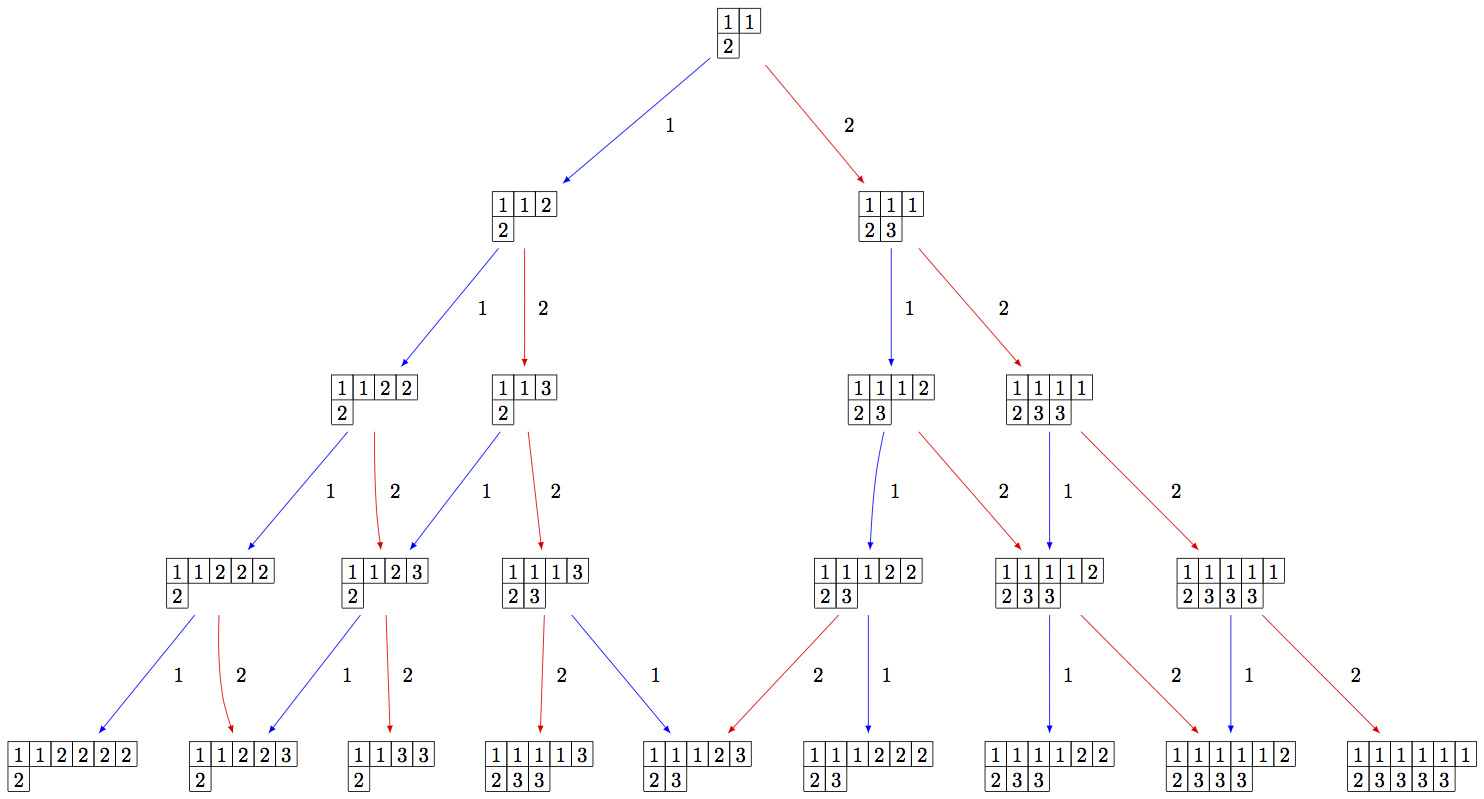
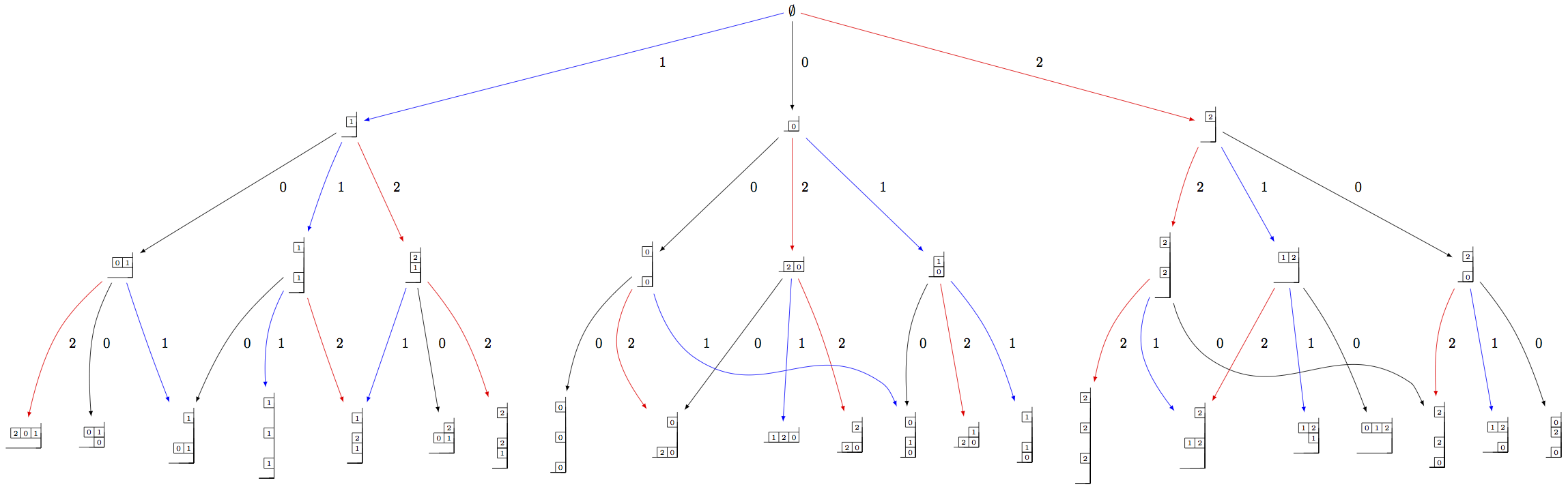
Since the crystal is infinite, we must specify the subcrystal we would like to view:
sage: B = crystals.infinity.Tableaux(['A',2])
sage: S = B.subcrystal(max_depth=4)
sage: G = B.digraph(subset=S)
sage: view(G, tightpage=True) # optional - dot2tex graphviz, not tested (opens external window)
>>> from sage.all import *
>>> B = crystals.infinity.Tableaux(['A',Integer(2)])
>>> S = B.subcrystal(max_depth=Integer(4))
>>> G = B.digraph(subset=S)
>>> view(G, tightpage=True) # optional - dot2tex graphviz, not tested (opens external window)
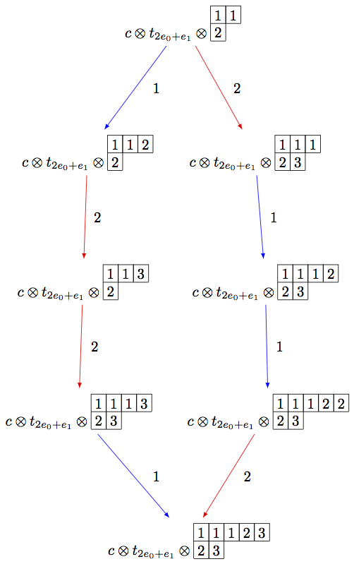
Using elementary crystals, we can cut irreducible highest weight crystals from \(B(\infty)\) as the connected component of \(C \otimes T_\lambda \otimes B(\infty)\) containing \(c\otimes t_\lambda \otimes u_\infty\), where \(u_\infty\) is the highest weight vector in \(B(\infty)\). In this example, we cut out \(B(\rho)\) from \(B(\infty)\) in type \(A_2\):
sage: B = crystals.infinity.Tableaux(['A',2])
sage: b = B.highest_weight_vector()
sage: T = crystals.elementary.T(['A',2], B.Lambda()[1] + B.Lambda()[2])
sage: t = T[0]
sage: C = crystals.elementary.Component(['A',2])
sage: c = C[0]
sage: TP = crystals.TensorProduct(C,T,B)
sage: t0 = TP(c,t,b)
sage: STP = TP.subcrystal(generators=[t0])
sage: GTP = TP.digraph(subset=STP)
sage: view(GTP, tightpage=True) # optional - dot2tex graphviz, not tested (opens external window)
>>> from sage.all import *
>>> B = crystals.infinity.Tableaux(['A',Integer(2)])
>>> b = B.highest_weight_vector()
>>> T = crystals.elementary.T(['A',Integer(2)], B.Lambda()[Integer(1)] + B.Lambda()[Integer(2)])
>>> t = T[Integer(0)]
>>> C = crystals.elementary.Component(['A',Integer(2)])
>>> c = C[Integer(0)]
>>> TP = crystals.TensorProduct(C,T,B)
>>> t0 = TP(c,t,b)
>>> STP = TP.subcrystal(generators=[t0])
>>> GTP = TP.digraph(subset=STP)
>>> view(GTP, tightpage=True) # optional - dot2tex graphviz, not tested (opens external window)
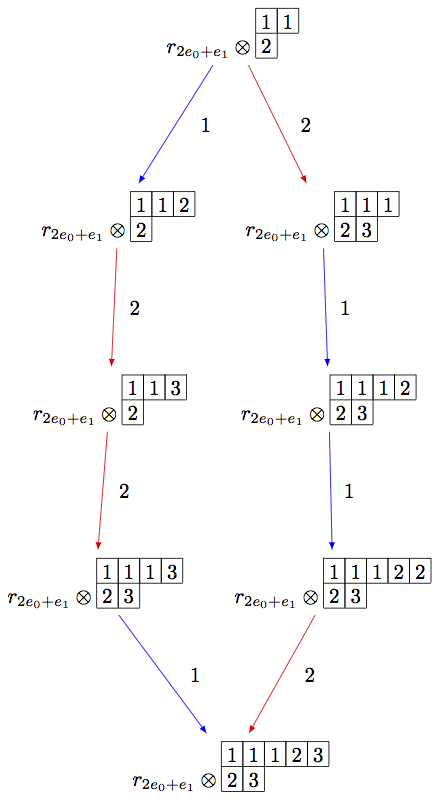
Note that the above code can be simplified using the R-crystal:
sage: B = crystals.infinity.Tableaux(['A',2])
sage: b = B.highest_weight_vector()
sage: R = crystals.elementary.R(['A',2], B.Lambda()[1] + B.Lambda()[2])
sage: r = R[0]
sage: TP2 = crystals.TensorProduct(R,B)
sage: t2 = TP2(r,b)
sage: STP2 = TP2.subcrystal(generators=[t2])
sage: GTP2 = TP2.digraph(subset=STP2)
sage: view(GTP2, tightpage=True) # optional - dot2tex graphviz, not tested (opens external window)
>>> from sage.all import *
>>> B = crystals.infinity.Tableaux(['A',Integer(2)])
>>> b = B.highest_weight_vector()
>>> R = crystals.elementary.R(['A',Integer(2)], B.Lambda()[Integer(1)] + B.Lambda()[Integer(2)])
>>> r = R[Integer(0)]
>>> TP2 = crystals.TensorProduct(R,B)
>>> t2 = TP2(r,b)
>>> STP2 = TP2.subcrystal(generators=[t2])
>>> GTP2 = TP2.digraph(subset=STP2)
>>> view(GTP2, tightpage=True) # optional - dot2tex graphviz, not tested (opens external window)
On the other hand, we can embed the irreducible highest weight crystal \(B(\rho)\) into \(B(\infty)\):
sage: Brho = crystals.Tableaux(['A',2],shape=[2,1])
sage: brho = Brho.highest_weight_vector()
sage: B = crystals.infinity.Tableaux(['A',2])
sage: binf = B.highest_weight_vector()
sage: wt = brho.weight()
sage: T = crystals.elementary.T(['A',2],wt)
sage: TlambdaBinf = crystals.TensorProduct(T,B)
sage: hw = TlambdaBinf(T[0],binf)
sage: Psi = Brho.crystal_morphism({brho : hw})
sage: BG = B.digraph(subset=[Psi(x) for x in Brho])
sage: view(BG, tightpage=True) # optional - dot2tex graphviz, not tested (opens external window)
>>> from sage.all import *
>>> Brho = crystals.Tableaux(['A',Integer(2)],shape=[Integer(2),Integer(1)])
>>> brho = Brho.highest_weight_vector()
>>> B = crystals.infinity.Tableaux(['A',Integer(2)])
>>> binf = B.highest_weight_vector()
>>> wt = brho.weight()
>>> T = crystals.elementary.T(['A',Integer(2)],wt)
>>> TlambdaBinf = crystals.TensorProduct(T,B)
>>> hw = TlambdaBinf(T[Integer(0)],binf)
>>> Psi = Brho.crystal_morphism({brho : hw})
>>> BG = B.digraph(subset=[Psi(x) for x in Brho])
>>> view(BG, tightpage=True) # optional - dot2tex graphviz, not tested (opens external window)
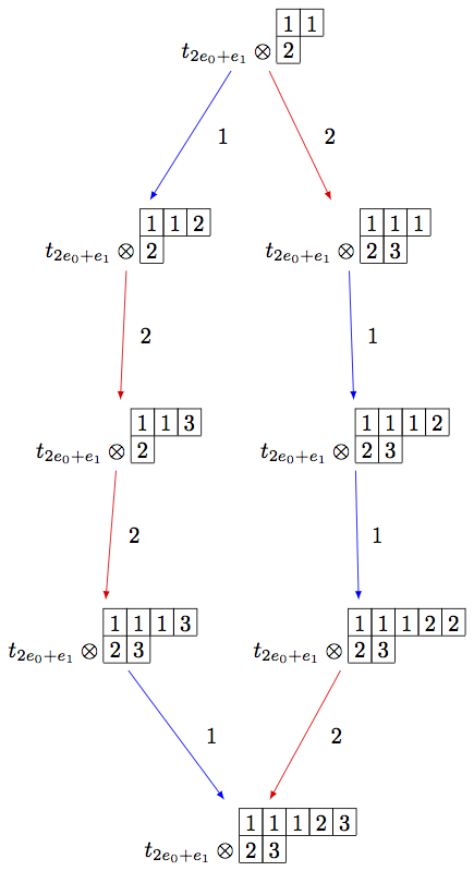
Note that in the last example, we had to inject \(B(\rho)\) into the tensor
product \(T_\lambda \otimes B(\infty)\), since otherwise, the map Psi would
not be a crystal morphism (as b.weight() != brho.weight()).
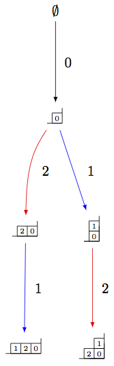
Generalized Young walls
Generalized Young walls were introduced by J.-A. Kim and D.-U. Shin as a model for \(B(\infty)\) and each \(B(\lambda)\) solely in affine type \(A_n^{(1)}\). See [KimShin2010] for more information on the construction of generalized Young walls.
Since this model is only valid for one Cartan type, the input to initialize the crystal is simply the rank of the underlying type:
sage: Y = crystals.infinity.GeneralizedYoungWalls(2)
sage: y = Y.highest_weight_vector()
sage: y.f_string([0,1,2,2,2,1,0,0,1,2]).pp()
         2|
          |
          |
       1|2|
       0|1|
 2|0|1|2|0|
>>> from sage.all import *
>>> Y = crystals.infinity.GeneralizedYoungWalls(Integer(2))
>>> y = Y.highest_weight_vector()
>>> y.f_string([Integer(0),Integer(1),Integer(2),Integer(2),Integer(2),Integer(1),Integer(0),Integer(0),Integer(1),Integer(2)]).pp()
         2|
          |
          |
       1|2|
       0|1|
 2|0|1|2|0|
In the weight method for this model, we can choose whether to view weights
in the extended weight lattice (by default) or in the root lattice:
sage: Y = crystals.infinity.GeneralizedYoungWalls(2)
sage: y = Y.highest_weight_vector()
sage: y.f_string([0,1,2,2,2,1,0,0,1,2]).weight()
Lambda[0] + Lambda[1] - 2*Lambda[2] - 3*delta
sage: y.f_string([0,1,2,2,2,1,0,0,1,2]).weight(root_lattice=True)
-3*alpha[0] - 3*alpha[1] - 4*alpha[2]
>>> from sage.all import *
>>> Y = crystals.infinity.GeneralizedYoungWalls(Integer(2))
>>> y = Y.highest_weight_vector()
>>> y.f_string([Integer(0),Integer(1),Integer(2),Integer(2),Integer(2),Integer(1),Integer(0),Integer(0),Integer(1),Integer(2)]).weight()
Lambda[0] + Lambda[1] - 2*Lambda[2] - 3*delta
>>> y.f_string([Integer(0),Integer(1),Integer(2),Integer(2),Integer(2),Integer(1),Integer(0),Integer(0),Integer(1),Integer(2)]).weight(root_lattice=True)
-3*alpha[0] - 3*alpha[1] - 4*alpha[2]
As before, we need to indicate a specific subcrystal when attempting to view the crystal graph:
sage: Y = crystals.infinity.GeneralizedYoungWalls(2)
sage: SY = Y.subcrystal(max_depth=3)
sage: GY = Y.digraph(subset=SY)
sage: view(GY, tightpage=True) # optional - dot2tex graphviz, not tested (opens external window)
>>> from sage.all import *
>>> Y = crystals.infinity.GeneralizedYoungWalls(Integer(2))
>>> SY = Y.subcrystal(max_depth=Integer(3))
>>> GY = Y.digraph(subset=SY)
>>> view(GY, tightpage=True) # optional - dot2tex graphviz, not tested (opens external window)
One can also make irreducible highest weight crystals using generalized Young walls:
sage: La = RootSystem(['A',2,1]).weight_lattice(extended=True).fundamental_weights()
sage: YLa = crystals.GeneralizedYoungWalls(2,La[0])
sage: SYLa = YLa.subcrystal(max_depth=3)
sage: GYLa = YLa.digraph(subset=SYLa)
sage: view(GYLa, tightpage=True) # optional - dot2tex graphviz, not tested (opens external window)
>>> from sage.all import *
>>> La = RootSystem(['A',Integer(2),Integer(1)]).weight_lattice(extended=True).fundamental_weights()
>>> YLa = crystals.GeneralizedYoungWalls(Integer(2),La[Integer(0)])
>>> SYLa = YLa.subcrystal(max_depth=Integer(3))
>>> GYLa = YLa.digraph(subset=SYLa)
>>> view(GYLa, tightpage=True) # optional - dot2tex graphviz, not tested (opens external window)
In the highest weight crystals, however, weights are always elements of the extended affine weight lattice:
sage: La = RootSystem(['A',2,1]).weight_lattice(extended=True).fundamental_weights()
sage: YLa = crystals.GeneralizedYoungWalls(2,La[0])
sage: YLa.highest_weight_vector().f_string([0,1,2,0]).weight()
-Lambda[0] + Lambda[1] + Lambda[2] - 2*delta
>>> from sage.all import *
>>> La = RootSystem(['A',Integer(2),Integer(1)]).weight_lattice(extended=True).fundamental_weights()
>>> YLa = crystals.GeneralizedYoungWalls(Integer(2),La[Integer(0)])
>>> YLa.highest_weight_vector().f_string([Integer(0),Integer(1),Integer(2),Integer(0)]).weight()
-Lambda[0] + Lambda[1] + Lambda[2] - 2*delta
Modified Nakajima monomials
Let \(Y_{i,k}\), for \(i \in I\) and \(k \in \ZZ\), be a commuting set of variables, and let \(\boldsymbol{1}\) be a new variable which commutes with each \(Y_{i,k}\). (Here, \(I\) represents the index set of a Cartan datum.) One may endow the structure of a crystal on the set \(\widehat{\mathcal{M}}\) of monomials of the form
Elements of \(\widehat{\mathcal{M}}\) are called modified Nakajima monomials. We will omit the \(\boldsymbol{1}\) from the end of a monomial if there exists at least one \(y_i(k) \neq 0\). The crystal structure on this set is defined by
where \(\{h_i : i \in I\}\) and \(\{\Lambda_i : i \in I \}\) are the simple coroots and fundamental weights, respectively. With a chosen set of integers \(C = (c_{ij})_{i\neq j}\) such that \(c_{ij}+c_{ji} =1\), one defines
where \((a_{ij})\) is a Cartan matrix. Then
Note
Monomial crystals depend on the choice of positive integers \(C = (c_{ij})_{i\neq j}\) satisfying the condition \(c_{ij}+c_{ji}=1\). This choice has been made in Sage such that \(c_{ij} = 1\) if \(i < j\) and \(c_{ij} = 0\) if \(i>j\), but other choices may be used if deliberately stated at the initialization of the crystal:
sage: c = Matrix([[0,0,1],[1,0,0],[0,1,0]])
sage: La = RootSystem(['C',3]).weight_lattice().fundamental_weights()
sage: M = crystals.NakajimaMonomials(2*La[1], c=c)
sage: M.c()
[0 0 1]
[1 0 0]
[0 1 0]
>>> from sage.all import *
>>> c = Matrix([[Integer(0),Integer(0),Integer(1)],[Integer(1),Integer(0),Integer(0)],[Integer(0),Integer(1),Integer(0)]])
>>> La = RootSystem(['C',Integer(3)]).weight_lattice().fundamental_weights()
>>> M = crystals.NakajimaMonomials(Integer(2)*La[Integer(1)], c=c)
>>> M.c()
[0 0 1]
[1 0 0]
[0 1 0]
It is shown in [KKS2007] that the connected component of \(\widehat{\mathcal{M}}\) containing the element \(\boldsymbol{1}\), which we denote by \(\mathcal{M}(\infty)\), is crystal isomorphic to the crystal \(B(\infty)\):
sage: Minf = crystals.infinity.NakajimaMonomials(['C',3,1])
sage: minf = Minf.highest_weight_vector()
sage: m = minf.f_string([0,1,2,3,2,1,0]); m
Y(0,0)^-1 Y(0,4)^-1 Y(1,0) Y(1,3)
sage: m.weight()
-2*Lambda[0] + 2*Lambda[1] - 2*delta
sage: m.weight_in_root_lattice()
-2*alpha[0] - 2*alpha[1] - 2*alpha[2] - alpha[3]
>>> from sage.all import *
>>> Minf = crystals.infinity.NakajimaMonomials(['C',Integer(3),Integer(1)])
>>> minf = Minf.highest_weight_vector()
>>> m = minf.f_string([Integer(0),Integer(1),Integer(2),Integer(3),Integer(2),Integer(1),Integer(0)]); m
Y(0,0)^-1 Y(0,4)^-1 Y(1,0) Y(1,3)
>>> m.weight()
-2*Lambda[0] + 2*Lambda[1] - 2*delta
>>> m.weight_in_root_lattice()
-2*alpha[0] - 2*alpha[1] - 2*alpha[2] - alpha[3]
We can also model \(B(\infty)\) using the variables \(A_{i,k}\) instead:
sage: Minf = crystals.infinity.NakajimaMonomials(['C',3,1])
sage: minf = Minf.highest_weight_vector()
sage: Minf.set_variables('A')
sage: m = minf.f_string([0,1,2,3,2,1,0]); m
A(0,0)^-1 A(0,3)^-1 A(1,0)^-1 A(1,2)^-1 A(2,0)^-1 A(2,1)^-1 A(3,0)^-1
sage: m.weight()
-2*Lambda[0] + 2*Lambda[1] - 2*delta
sage: m.weight_in_root_lattice()
-2*alpha[0] - 2*alpha[1] - 2*alpha[2] - alpha[3]
sage: Minf.set_variables('Y')
>>> from sage.all import *
>>> Minf = crystals.infinity.NakajimaMonomials(['C',Integer(3),Integer(1)])
>>> minf = Minf.highest_weight_vector()
>>> Minf.set_variables('A')
>>> m = minf.f_string([Integer(0),Integer(1),Integer(2),Integer(3),Integer(2),Integer(1),Integer(0)]); m
A(0,0)^-1 A(0,3)^-1 A(1,0)^-1 A(1,2)^-1 A(2,0)^-1 A(2,1)^-1 A(3,0)^-1
>>> m.weight()
-2*Lambda[0] + 2*Lambda[1] - 2*delta
>>> m.weight_in_root_lattice()
-2*alpha[0] - 2*alpha[1] - 2*alpha[2] - alpha[3]
>>> Minf.set_variables('Y')
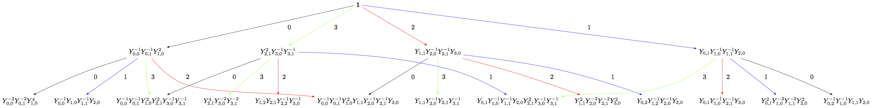
Building the crystal graph output for these monomial crystals is the same as the constructions above:
sage: Minf = crystals.infinity.NakajimaMonomials(['C',3,1])
sage: Sinf = Minf.subcrystal(max_depth=2)
sage: Ginf = Minf.digraph(subset=Sinf)
sage: view(Ginf, tightpage=True) # optional - dot2tex graphviz, not tested (opens external window)
>>> from sage.all import *
>>> Minf = crystals.infinity.NakajimaMonomials(['C',Integer(3),Integer(1)])
>>> Sinf = Minf.subcrystal(max_depth=Integer(2))
>>> Ginf = Minf.digraph(subset=Sinf)
>>> view(Ginf, tightpage=True) # optional - dot2tex graphviz, not tested (opens external window)
Note that this model will also work for any symmetrizable Cartan matrix:
sage: A = CartanMatrix([[2,-4],[-5,2]])
sage: Linf = crystals.infinity.NakajimaMonomials(A); Linf
Infinity Crystal of modified Nakajima monomials of type [ 2 -4]
[-5  2]
sage: Linf.highest_weight_vector().f_string([0,1,1,1,0,0,1,1,0])
Y(0,0)^-1 Y(0,1)^9 Y(0,2)^5 Y(0,3)^-1 Y(1,0)^2 Y(1,1)^5 Y(1,2)^3
>>> from sage.all import *
>>> A = CartanMatrix([[Integer(2),-Integer(4)],[-Integer(5),Integer(2)]])
>>> Linf = crystals.infinity.NakajimaMonomials(A); Linf
Infinity Crystal of modified Nakajima monomials of type [ 2 -4]
[-5  2]
>>> Linf.highest_weight_vector().f_string([Integer(0),Integer(1),Integer(1),Integer(1),Integer(0),Integer(0),Integer(1),Integer(1),Integer(0)])
Y(0,0)^-1 Y(0,1)^9 Y(0,2)^5 Y(0,3)^-1 Y(1,0)^2 Y(1,1)^5 Y(1,2)^3
Rigged configurations
Rigged configurations are sequences of partitions, one partition for each node in the underlying Dynkin diagram, such that each part of each partition has a label (or rigging). A crystal structure was defined on these objects in [Schilling2006], then later extended to work as a model for \(B(\infty)\). See [SalisburyScrimshaw2015] for more information:
sage: RiggedConfigurations.options(display="horizontal")
sage: RC = crystals.infinity.RiggedConfigurations(['C',3,1])
sage: nu = RC.highest_weight_vector().f_string([0,1,2,3,2,1,0]); nu
-2[ ]-1   2[ ]1   0[ ]0   0[ ]0
-2[ ]-1   2[ ]1   0[ ]0
sage: nu.weight()
-2*Lambda[0] + 2*Lambda[1] - 2*delta
sage: RiggedConfigurations.options._reset()
>>> from sage.all import *
>>> RiggedConfigurations.options(display="horizontal")
>>> RC = crystals.infinity.RiggedConfigurations(['C',Integer(3),Integer(1)])
>>> nu = RC.highest_weight_vector().f_string([Integer(0),Integer(1),Integer(2),Integer(3),Integer(2),Integer(1),Integer(0)]); nu
-2[ ]-1   2[ ]1   0[ ]0   0[ ]0
-2[ ]-1   2[ ]1   0[ ]0
>>> nu.weight()
-2*Lambda[0] + 2*Lambda[1] - 2*delta
>>> RiggedConfigurations.options._reset()
We can check this crystal is isomorphic to the crystal above using Nakajima monomials:
sage: Minf = crystals.infinity.NakajimaMonomials(['C',3,1])
sage: Sinf = Minf.subcrystal(max_depth=2)
sage: Ginf = Minf.digraph(subset=Sinf)
sage: RC = crystals.infinity.RiggedConfigurations(['C',3,1])
sage: RCS = RC.subcrystal(max_depth=2)
sage: RCG = RC.digraph(subset=RCS)
sage: RCG.is_isomorphic(Ginf, edge_labels=True)
True
>>> from sage.all import *
>>> Minf = crystals.infinity.NakajimaMonomials(['C',Integer(3),Integer(1)])
>>> Sinf = Minf.subcrystal(max_depth=Integer(2))
>>> Ginf = Minf.digraph(subset=Sinf)
>>> RC = crystals.infinity.RiggedConfigurations(['C',Integer(3),Integer(1)])
>>> RCS = RC.subcrystal(max_depth=Integer(2))
>>> RCG = RC.digraph(subset=RCS)
>>> RCG.is_isomorphic(Ginf, edge_labels=True)
True
This model works in Sage for all finite and affine types, as well as any simply laced Cartan matrix.