Abelian Sandpile Model
Author: David Perkinson, Reed College
Introduction
These notes provide an introduction to Dhar’s abelian sandpile model (ASM) and to Sage Sandpiles, a collection of tools in Sage for doing sandpile calculations. For a more thorough introduction to the theory of the ASM, the papers Chip-Firing and Rotor-Routing on Directed Graphs [H] by Holroyd et al., and Riemann-Roch and Abel-Jacobi Theory on a Finite Graph by Baker and Norine [BN] are recommended. See also [PPW2013].
To describe the ASM, we start with a sandpile graph: a directed multigraph \(\Gamma\) with a vertex \(s\) that is accessible from every vertex. By multigraph, we mean that each edge of \(\Gamma\) is assigned a nonnegative integer weight. To say \(s\) is accessible from some vertex \(v\) means that there is a sequence (possibly empty) of directed edges starting at \(v\) and ending at \(s\). We call \(s\) the sink of the sandpile graph, even though it might have outgoing edges, for reasons that will be made clear in a moment.
We denote the vertex set of \(\Gamma\) by \(V\), and define \(\tilde{V} = V\setminus\{s\}\). For any vertex \(v\), we let \(\mbox{out-degree}(v)\) (the out-degree of \(v\)) be the sum of the weights of all edges leaving \(v\).
Configurations and divisors
A configuration on \(\Gamma\) is an element of \(\ZZ_{\geq 0} \tilde{V}\), i.e., the assignment of a nonnegative integer to each nonsink vertex. We think of each integer as a number of grains of sand being placed at the corresponding vertex. A divisor on \(\Gamma\) is an element of \(\ZZ V\), i.e., an element in the free abelian group on all of the vertices. In the context of divisors, it is sometimes useful to think of a divisor on \(\Gamma\) as assigning dollars to each vertex, with negative integers signifying a debt.
Stabilization
A configuration \(c\) is stable at a vertex \(v\in\tilde{V}\) if \(c(v) < \mbox{out-degree}(v)\). Otherwise, \(c\) is unstable at \(v\). A configuration \(c\) (in itself) is stable if it is stable at each nonsink vertex. Otherwise, \(c\) is unstable. If \(c\) is unstable at \(v\), the vertex \(v\) can be fired (toppled) by removing \(\mbox{out-degree}(v)\) grains of sand from \(v\) and adding grains of sand to the neighbors of \(v\), determined by the weights of the edges leaving \(v\) (each vertex \(w\) gets as many grains as the weight of the edge \((v, w)\) is, if there is such an edge). Note that grains that are added to the sink \(s\) are not counted (i.e., they “disappear”).
Despite our best intentions, we sometimes consider firing a stable vertex, resulting in a “configuration” with a negative amount of sand at that vertex. We may also reverse-fire a vertex, absorbing sand from the vertex’s neighbors (including the sink).
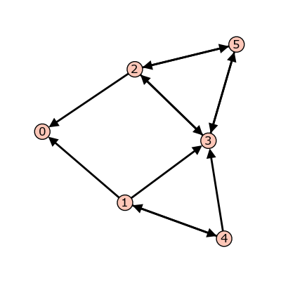
Example. Consider the graph:
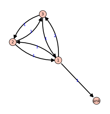
\(\Gamma\)
All edges have weight \(1\) except for the edge from vertex 1 to vertex 3, which has weight \(2\). If we let \(c = (5,0,1)\) with the indicated number of grains of sand on vertices 1, 2, and 3, respectively, then only vertex 1, whose out-degree is 4, is unstable. Firing vertex 1 gives a new configuration \(c' = (1,1,3)\). Here, \(4\) grains have left vertex 1. One of these has gone to the sink vertex (and forgotten), one has gone to vertex 2, and two have gone to vertex 3, since the edge from 1 to 3 has weight \(2\). Vertex 3 in the new configuration is now unstable. The Sage code for this example follows.
sage: g = {0:{},
....:      1:{0:1, 2:1, 3:2},
....:      2:{1:1, 3:1},
....:      3:{1:1, 2:1}}
sage: S = Sandpile(g, 0)   # create the sandpile
sage: S.show(edge_labels=true)  # display the graph
>>> from sage.all import *
>>> g = {Integer(0):{},
...      Integer(1):{Integer(0):Integer(1), Integer(2):Integer(1), Integer(3):Integer(2)},
...      Integer(2):{Integer(1):Integer(1), Integer(3):Integer(1)},
...      Integer(3):{Integer(1):Integer(1), Integer(2):Integer(1)}}
>>> S = Sandpile(g, Integer(0))   # create the sandpile
>>> S.show(edge_labels=true)  # display the graph
Create the configuration:
sage: c = SandpileConfig(S, {1:5, 2:0, 3:1})
sage: S.out_degree()
{0: 0, 1: 4, 2: 2, 3: 2}
>>> from sage.all import *
>>> c = SandpileConfig(S, {Integer(1):Integer(5), Integer(2):Integer(0), Integer(3):Integer(1)})
>>> S.out_degree()
{0: 0, 1: 4, 2: 2, 3: 2}
Fire vertex \(1\):
sage: c.fire_vertex(1)
{1: 1, 2: 1, 3: 3}
>>> from sage.all import *
>>> c.fire_vertex(Integer(1))
{1: 1, 2: 1, 3: 3}
The configuration is unchanged:
sage: c
{1: 5, 2: 0, 3: 1}
>>> from sage.all import *
>>> c
{1: 5, 2: 0, 3: 1}
Repeatedly fire vertices until the configuration becomes stable:
sage: c.stabilize()
{1: 2, 2: 1, 3: 1}
>>> from sage.all import *
>>> c.stabilize()
{1: 2, 2: 1, 3: 1}
Alternatives:
sage: ~c             # shorthand for c.stabilize()
{1: 2, 2: 1, 3: 1}
sage: c.stabilize(with_firing_vector=true)
[{1: 2, 2: 1, 3: 1}, {1: 2, 2: 2, 3: 3}]
>>> from sage.all import *
>>> ~c             # shorthand for c.stabilize()
{1: 2, 2: 1, 3: 1}
>>> c.stabilize(with_firing_vector=true)
[{1: 2, 2: 1, 3: 1}, {1: 2, 2: 2, 3: 3}]
Since vertex 3 has become unstable after firing vertex 1, it can be fired, which causes vertex 2 to become unstable, etc. Repeated firings eventually lead to a stable configuration. The last line of the Sage code, above, is a list, the first element of which is the resulting stable configuration, \((2,1,1)\). The second component records how many times each vertex fired in the stabilization.
Since the sink is accessible from each nonsink vertex and never fires, every configuration will stabilize after a finite number of vertex-firings. It is not obvious, but the resulting stabilization is independent of the order in which unstable vertices are fired. Thus, each configuration stabilizes to a unique stable configuration.
Laplacian
Fix a total order on the vertices of \(\Gamma\), thus leading to a labelling of the vertices by the numbers \(1, 2, \ldots, n\) for some \(n\) (in the given order). The Laplacian of \(\Gamma\) is
where \(D\) is the diagonal matrix of out-degrees of the vertices (i.e., the diagonal \(n \times n\)-matrix whose \((i, i)\)-th entry is the out-degree of the vertex \(i\)) and \(A\) is the adjacency matrix whose \((i,j)\)-th entry is the weight of the edge from vertex \(i\) to vertex \(j\), which we take to be \(0\) if there is no edge. The reduced Laplacian, \(\tilde{L}\), is the submatrix of the Laplacian formed by removing the row and column corresponding to the sink vertex. Firing a vertex of a configuration is the same as subtracting the corresponding row of the reduced Laplacian.
Example. (Continued.)
sage: S.vertices(sort=True)  # the ordering of the vertices
[0, 1, 2, 3]
sage: S.laplacian()
[ 0  0  0  0]
[-1  4 -1 -2]
[ 0 -1  2 -1]
[ 0 -1 -1  2]
sage: S.reduced_laplacian()
[ 4 -1 -2]
[-1  2 -1]
[-1 -1  2]
>>> from sage.all import *
>>> S.vertices(sort=True)  # the ordering of the vertices
[0, 1, 2, 3]
>>> S.laplacian()
[ 0  0  0  0]
[-1  4 -1 -2]
[ 0 -1  2 -1]
[ 0 -1 -1  2]
>>> S.reduced_laplacian()
[ 4 -1 -2]
[-1  2 -1]
[-1 -1  2]
The configuration we considered previously:
sage: c = SandpileConfig(S, [5,0,1])
sage: c
{1: 5, 2: 0, 3: 1}
>>> from sage.all import *
>>> c = SandpileConfig(S, [Integer(5),Integer(0),Integer(1)])
>>> c
{1: 5, 2: 0, 3: 1}
Firing vertex 1 is the same as subtracting the corresponding row of the reduced Laplacian from the configuration (regarded as a vector):
sage: c.fire_vertex(1).values()
[1, 1, 3]
sage: S.reduced_laplacian()[0]
(4, -1, -2)
sage: vector([5,0,1]) - vector([4,-1,-2])
(1, 1, 3)
>>> from sage.all import *
>>> c.fire_vertex(Integer(1)).values()
[1, 1, 3]
>>> S.reduced_laplacian()[Integer(0)]
(4, -1, -2)
>>> vector([Integer(5),Integer(0),Integer(1)]) - vector([Integer(4),-Integer(1),-Integer(2)])
(1, 1, 3)
Recurrent elements
Imagine an experiment in which grains of sand are dropped one-at-a-time onto a graph, pausing to allow the configuration to stabilize between drops. Some configurations will only be seen once in this process. For example, for most graphs, once sand is dropped on the graph, no sequence of additions of sand and stabilizations will result in a graph empty of sand. Other configurations—the so-called recurrent configurations—will be seen infinitely often as the process is repeated indefinitely.
To be precise, a configuration \(c\) is recurrent if (i) it is stable, and (ii) given any configuration \(a\), there is a configuration \(b\) such that \(c = \mbox{stab}(a+b)\), the stabilization of \(a + b\).
The maximal-stable configuration, denoted \(c_{\mathrm{max}}\), is defined by \(c_{\mathrm{max}}(v)=\mbox{out-degree}(v)-1\) for all nonsink vertices \(v\). It is clear that \(c_{\mathrm{max}}\) is recurrent. Further, it is not hard to see that a configuration is recurrent if and only if it has the form \(\mbox{stab}(a+c_{\mathrm{max}})\) for some configuration \(a\).
Example. (Continued.)
sage: S.recurrents(verbose=false)
[[3, 1, 1], [2, 1, 1], [3, 1, 0]]
sage: c = SandpileConfig(S, [2,1,1])
sage: c
{1: 2, 2: 1, 3: 1}
sage: c.is_recurrent()
True
sage: S.max_stable()
{1: 3, 2: 1, 3: 1}
>>> from sage.all import *
>>> S.recurrents(verbose=false)
[[3, 1, 1], [2, 1, 1], [3, 1, 0]]
>>> c = SandpileConfig(S, [Integer(2),Integer(1),Integer(1)])
>>> c
{1: 2, 2: 1, 3: 1}
>>> c.is_recurrent()
True
>>> S.max_stable()
{1: 3, 2: 1, 3: 1}
Adding any configuration to the max-stable configuration and stabilizing yields a recurrent configuration:
sage: x = SandpileConfig(S, [1,0,0])
sage: x + S.max_stable()
{1: 4, 2: 1, 3: 1}
>>> from sage.all import *
>>> x = SandpileConfig(S, [Integer(1),Integer(0),Integer(0)])
>>> x + S.max_stable()
{1: 4, 2: 1, 3: 1}
Use & to add and stabilize:
sage: c = x & S.max_stable()
sage: c
{1: 3, 2: 1, 3: 0}
sage: c.is_recurrent()
True
>>> from sage.all import *
>>> c = x & S.max_stable()
>>> c
{1: 3, 2: 1, 3: 0}
>>> c.is_recurrent()
True
Note the various ways of performing addition and stabilization:
sage: m = S.max_stable()
sage: (x + m).stabilize() == ~(x + m)
True
sage: (x + m).stabilize() == x & m
True
>>> from sage.all import *
>>> m = S.max_stable()
>>> (x + m).stabilize() == ~(x + m)
True
>>> (x + m).stabilize() == x & m
True
Burning Configuration
A burning configuration is a \(\ZZ_{\geq 0}\)-linear combination \(f\) of the rows of the reduced Laplacian matrix having nonnegative entries and such that every vertex is accessible from some vertex in the support of \(f\) (in other words, for each vertex \(w\), there is a path from some \(v \in \operatorname{supp} f\) to \(w\)). The corresponding burning script gives the coefficients in the \(\ZZ_{\geq 0}\)-linear combination needed to obtain the burning configuration. So if \(b\) is a burning configuration, \(\sigma\) is its script, and \(\tilde{L}\) is the reduced Laplacian, then \(\sigma\,\tilde{L} = b\). The minimal burning configuration is the one with the minimal script (each of its components is no larger than the corresponding component of any other script for a burning configuration).
Given a burning configuration \(b\) having script \(\sigma\), and any configuration \(c\) on the same graph, the following are equivalent:
\(c\) is recurrent;
\(c + b\) stabilizes to \(c\);
the firing vector for the stabilization of \(c + b\) is \(\sigma\).
The burning configuration and script are computed using a modified version of Speer’s script algorithm. This is a generalization to directed multigraphs of Dhar’s burning algorithm.
Example.
sage: g = {0:{},1:{0:1,3:1,4:1},2:{0:1,3:1,5:1},
....:      3:{2:1,5:1},4:{1:1,3:1},5:{2:1,3:1}}
sage: G = Sandpile(g,0)
sage: G.burning_config()
{1: 2, 2: 0, 3: 1, 4: 1, 5: 0}
sage: G.burning_config().values()
[2, 0, 1, 1, 0]
sage: G.burning_script()
{1: 1, 2: 3, 3: 5, 4: 1, 5: 4}
sage: G.burning_script().values()
[1, 3, 5, 1, 4]
sage: matrix(G.burning_script().values())*G.reduced_laplacian()
[2 0 1 1 0]
>>> from sage.all import *
>>> g = {Integer(0):{},Integer(1):{Integer(0):Integer(1),Integer(3):Integer(1),Integer(4):Integer(1)},Integer(2):{Integer(0):Integer(1),Integer(3):Integer(1),Integer(5):Integer(1)},
...      Integer(3):{Integer(2):Integer(1),Integer(5):Integer(1)},Integer(4):{Integer(1):Integer(1),Integer(3):Integer(1)},Integer(5):{Integer(2):Integer(1),Integer(3):Integer(1)}}
>>> G = Sandpile(g,Integer(0))
>>> G.burning_config()
{1: 2, 2: 0, 3: 1, 4: 1, 5: 0}
>>> G.burning_config().values()
[2, 0, 1, 1, 0]
>>> G.burning_script()
{1: 1, 2: 3, 3: 5, 4: 1, 5: 4}
>>> G.burning_script().values()
[1, 3, 5, 1, 4]
>>> matrix(G.burning_script().values())*G.reduced_laplacian()
[2 0 1 1 0]
Sandpile group
The collection of stable configurations forms a commutative monoid with addition defined as ordinary addition followed by stabilization. The identity element is the all-zero configuration. This monoid is a group exactly when the underlying graph is a DAG (directed acyclic graph).
The recurrent elements form a submonoid which turns out to be a group. This group is called the sandpile group for \(\Gamma\), denoted \(\mathcal{S}(\Gamma)\). Its identity element is usually not the all-zero configuration (again, only in the case that \(\Gamma\) is a DAG). So finding the identity element is an interesting problem.
Let \(n=|V|-1\) and fix an ordering of the nonsink vertices. Let \(\mathcal{\tilde{L}}\subset\ZZ^n\) denote the column-span of \(\tilde{L}^t\), the transpose of the reduced Laplacian. It is a theorem that
Thus, the number of elements of the sandpile group is \(\det{\tilde{L}}\), which by the matrix-tree theorem is the number of weighted trees directed into the sink.
Example. (Continued.)
sage: S.group_order()
3
sage: S.invariant_factors()
[1, 1, 3]
sage: S.reduced_laplacian().dense_matrix().smith_form()
(
[1 0 0]  [ 1  0  0]  [1 3 5]
[0 1 0]  [ 0  1  0]  [1 4 6]
[0 0 3], [ 0 -1  1], [1 4 7]
)
>>> from sage.all import *
>>> S.group_order()
3
>>> S.invariant_factors()
[1, 1, 3]
>>> S.reduced_laplacian().dense_matrix().smith_form()
(
[1 0 0]  [ 1  0  0]  [1 3 5]
[0 1 0]  [ 0  1  0]  [1 4 6]
[0 0 3], [ 0 -1  1], [1 4 7]
)
Adding the identity to any recurrent configuration and stabilizing yields the same recurrent configuration:
sage: S.identity()
{1: 3, 2: 1, 3: 0}
sage: i = S.identity()
sage: m = S.max_stable()
sage: i & m == m
True
>>> from sage.all import *
>>> S.identity()
{1: 3, 2: 1, 3: 0}
>>> i = S.identity()
>>> m = S.max_stable()
>>> i & m == m
True
Self-organized criticality
The sandpile model was introduced by Bak, Tang, and Wiesenfeld in the paper, Self-organized criticality: an explanation of 1/ƒ noise [BTW]. The term self-organized criticality has no precise definition, but can be loosely taken to describe a system that naturally evolves to a state that is barely stable and such that the instabilities are described by a power law. In practice, self-organized criticality is often taken to mean like the sandpile model on a grid graph. The grid graph is just a grid with an extra sink vertex. The vertices on the interior of each side have one edge to the sink, and the corner vertices have an edge of weight \(2\). Thus, every nonsink vertex has out-degree \(4\).
Imagine repeatedly dropping grains of sand on an empty grid graph, allowing the sandpile to stabilize in between. At first there is little activity, but as time goes on, the size and extent of the avalanche caused by a single grain of sand becomes hard to predict. Computer experiments—I do not think there is a proof, yet—indicate that the distribution of avalanche sizes obeys a power law with exponent -1. In the example below, the size of an avalanche is taken to be the sum of the number of times each vertex fires.
Example (distribution of avalanche sizes).
sage: S = sandpiles.Grid(10,10)
sage: m = S.max_stable()
sage: a = []
sage: for i in range(10000):  # long time (15s on sage.math, 2012)
....:     m = m.add_random()
....:     m, f = m.stabilize(true)
....:     a.append(sum(f.values()))
...
sage: p = list_plot([[log(i+1),log(a.count(i))] for i in [0..max(a)] if a.count(i)])  # long time
sage: p.axes_labels(['log(N)','log(D(N))'])  # long time
sage: p  # long time
Graphics object consisting of 1 graphics primitive
>>> from sage.all import *
>>> S = sandpiles.Grid(Integer(10),Integer(10))
>>> m = S.max_stable()
>>> a = []
>>> for i in range(Integer(10000)):  # long time (15s on sage.math, 2012)
...     m = m.add_random()
...     m, f = m.stabilize(true)
...     a.append(sum(f.values()))
...
>>> p = list_plot([[log(i+Integer(1)),log(a.count(i))] for i in (ellipsis_range(Integer(0),Ellipsis,max(a))) if a.count(i)])  # long time
>>> p.axes_labels(['log(N)','log(D(N))'])  # long time
>>> p  # long time
Graphics object consisting of 1 graphics primitive
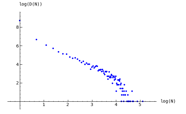
Distribution of avalanche sizes
Note: In the above code, m.stabilize(true) returns a list consisting of the
stabilized configuration and the firing vector. (Omitting true would give
just the stabilized configuration.)
Divisors and Discrete Riemann surfaces
A reference for this section is Riemann-Roch and Abel-Jacobi theory on a finite graph [BN].
A divisor on \(\Gamma\) is an element of the free abelian group on its vertices, including the sink. Suppose, as above, that the \(n+1\) vertices of \(\Gamma\) have been ordered, and that \(\mathcal{L}\) is the column span of the transpose of the Laplacian. A divisor is then identified with an element \(D\in\ZZ^{n+1}\), and two divisors are linearly equivalent if they differ by an element of \(\mathcal{L}\). A divisor \(E\) is effective, written \(E\geq0\), if \(E(v)\geq0\) for each \(v\in V\), i.e., if \(E\in\mathbb{Z}_{\geq 0}^{n+1}\). The degree of a divisor \(D\) is \(\deg(D) := \sum_{v\in V} D(v)\). The divisors of degree zero modulo linear equivalence form the Picard group, or Jacobian of the graph. For an undirected graph, the Picard group is isomorphic to the sandpile group.
The complete linear system for a divisor \(D\), denoted \(|D|\), is the collection of effective divisors linearly equivalent to \(D\).
Riemann-Roch
To describe the Riemann-Roch theorem in this context, suppose that \(\Gamma\) is an undirected, unweighted graph. The dimension, \(r(D)\), of the linear system \(|D|\) is \(-1\) if \(|D|=\emptyset\), and otherwise is the greatest integer \(s\) such that \(|D-E|\neq0\) for all effective divisors \(E\) of degree \(s\). Define the canonical divisor by \(K = \sum_{v\in V} (\deg(v)-2) v\), and the genus by \(g = \#(E) - \#(V) + 1\). The Riemann-Roch theorem says that for any divisor \(D\),
Example.
sage: G = sandpiles.Complete(5) # the sandpile on the complete graph with 5 vertices
>>> from sage.all import *
>>> G = sandpiles.Complete(Integer(5))  # the sandpile on the complete graph with 5 vertices
A divisor on the graph:
sage: D = SandpileDivisor(G, [1,2,2,0,2])
>>> from sage.all import *
>>> D = SandpileDivisor(G, [Integer(1),Integer(2),Integer(2),Integer(0),Integer(2)])
Verify the Riemann-Roch theorem:
sage: K = G.canonical_divisor()
sage: D.rank() - (K - D).rank() == D.deg() + 1 - G.genus()
True
>>> from sage.all import *
>>> K = G.canonical_divisor()
>>> D.rank() - (K - D).rank() == D.deg() + Integer(1) - G.genus()
True
The effective divisors linearly equivalent to \(D\):
sage: D.effective_div(False)
[[0, 1, 1, 4, 1], [1, 2, 2, 0, 2], [4, 0, 0, 3, 0]]
>>> from sage.all import *
>>> D.effective_div(False)
[[0, 1, 1, 4, 1], [1, 2, 2, 0, 2], [4, 0, 0, 3, 0]]
The nonspecial divisors up to linear equivalence (divisors of degree \(g-1\) with empty linear systems):
sage: N = G.nonspecial_divisors()
sage: [E.values() for E in N[:5]]   # the first few
[[-1, 0, 1, 2, 3],
 [-1, 0, 1, 3, 2],
 [-1, 0, 2, 1, 3],
 [-1, 0, 2, 3, 1],
 [-1, 0, 3, 1, 2]]
sage: len(N)
24
sage: len(N) == G.h_vector()[-1]
True
>>> from sage.all import *
>>> N = G.nonspecial_divisors()
>>> [E.values() for E in N[:Integer(5)]]   # the first few
[[-1, 0, 1, 2, 3],
 [-1, 0, 1, 3, 2],
 [-1, 0, 2, 1, 3],
 [-1, 0, 2, 3, 1],
 [-1, 0, 3, 1, 2]]
>>> len(N)
24
>>> len(N) == G.h_vector()[-Integer(1)]
True
Picturing linear systems
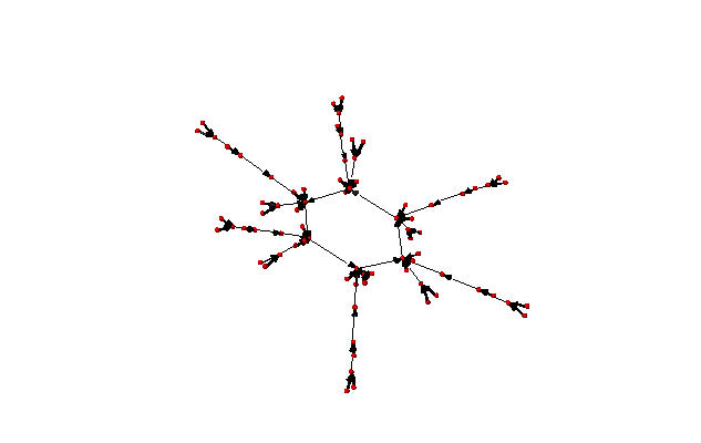
Fix a divisor \(D\). There are at least two natural graphs associated with the linear system associated with \(D\). First, consider the directed graph with vertex set \(|D|\) and with an edge from vertex \(E\) to vertex \(F\) if \(F\) is attained from \(E\) by firing a single unstable vertex.
sage: S = Sandpile(graphs.CycleGraph(6),0)
sage: D = SandpileDivisor(S, [1,1,1,1,2,0])
sage: D.is_alive()
True
sage: eff = D.effective_div()
sage: firing_graph(S,eff).show3d(edge_size=.005,vertex_size=0.01,iterations=500)
>>> from sage.all import *
>>> S = Sandpile(graphs.CycleGraph(Integer(6)),Integer(0))
>>> D = SandpileDivisor(S, [Integer(1),Integer(1),Integer(1),Integer(1),Integer(2),Integer(0)])
>>> D.is_alive()
True
>>> eff = D.effective_div()
>>> firing_graph(S,eff).show3d(edge_size=RealNumber('.005'),vertex_size=RealNumber('0.01'),iterations=Integer(500))
Complete linear system for \((1,1,1,1,2,0)\) on \(C_6\): single firings
The is_alive method checks whether the divisor \(D\) is alive, i.e.,
whether every divisor linearly equivalent to \(D\) is unstable.
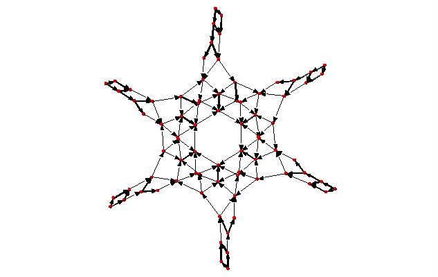
The second graph has the same set of vertices but with an edge from \(E\) to \(F\) if \(F\) is obtained from \(E\) by firing all unstable vertices of \(E\).
sage: S = Sandpile(graphs.CycleGraph(6),0)
sage: D = SandpileDivisor(S, [1,1,1,1,2,0])
sage: eff = D.effective_div()
sage: parallel_firing_graph(S,eff).show3d(edge_size=.005,vertex_size=0.01,iterations=500)
>>> from sage.all import *
>>> S = Sandpile(graphs.CycleGraph(Integer(6)),Integer(0))
>>> D = SandpileDivisor(S, [Integer(1),Integer(1),Integer(1),Integer(1),Integer(2),Integer(0)])
>>> eff = D.effective_div()
>>> parallel_firing_graph(S,eff).show3d(edge_size=RealNumber('.005'),vertex_size=RealNumber('0.01'),iterations=Integer(500))
Complete linear system for \((1,1,1,1,2,0)\) on \(C_6\): parallel firings
Note that in each of the examples above, starting at any divisor in the
linear system and following edges, one is eventually led into a cycle of
length \(6\) (cycling the divisor \((1,1,1,1,2,0)\)). Thus, D.alive()
returns True. In Sage, one would be able to rotate the above figures
to get a better idea of the structure.
Algebraic geometry of sandpiles
Affine
Let \(n = |V| - 1\), and fix an ordering on the nonsink vertices of \(\Gamma\). Let \(\tilde{\mathcal{L}} \subset \ZZ^n\) denote the column-span of \(\tilde{L}^t\), the transpose of the reduced Laplacian. Label vertex \(i\) with the indeterminate \(x_i\), and let \(\CC[\Gamma_s] = \CC[x_1, \dots, x_n]\). (Here, \(s\) denotes the sink vertex of \(\Gamma\).) The sandpile ideal or toppling ideal, first studied by Cori, Rossin, and Salvy [CRS] for undirected graphs, is the lattice ideal for \(\tilde{\mathcal{L}}\):
where \(x^u := \prod_{i=1}^n x^{u_i}\) for \(u \in \ZZ^n\).
For each \(c\in\ZZ^n\) define \(t(c) = x^{c^+} - x^{c^-}\) where \(c^+_i = \max\{c_i,0\}\) and \(c^-_i = \max\{-c_i,0\}\), so that \(c = c^+ - c^-\). Then, for each \(\sigma \in \ZZ^n\), define \(T(\sigma) = t(\tilde{L}^t\sigma)\). It then turns out that
where \(e_i\) is the \(i\)-th standard basis vector and \(b\) is any burning configuration.
The affine coordinate ring, \(\CC[\Gamma_s]/I,\) is isomorphic to the group algebra of the sandpile group, \(\CC[\mathcal{S}(\Gamma)]\).
The standard term-ordering on \(\CC[\Gamma_s]\) is graded reverse lexicographical order with \(x_i > x_j\) if vertex \(v_i\) is further from the sink than vertex \(v_j\). (There are choices to be made for vertices equidistant from the sink.) If \(\sigma_b\) is the script for a burning configuration (not necessarily minimal), then
is a Gröbner basis for \(I\).
Projective
Now let \(\CC[\Gamma] = \CC[x_0,x_1,\dots,x_n]\), where \(x_0\) corresponds to the sink vertex. The homogeneous sandpile ideal, denoted \(I^h\), is obtaining by homogenizing \(I\) with respect to \(x_0\). Let \(L\) be the (full) Laplacian, and \(\mathcal{L} \subset \ZZ^{n+1}\) be the column span of its transpose, \(L^t.\) Then \(I^h\) is the lattice ideal for \(\mathcal{L}\):
This ideal can be calculated by saturating the ideal
with respect to the product of the indeterminates: \(\prod_{i=0}^n x_i\) (extending the \(T\) operator in the obvious way). A Gröbner basis with respect to the degree lexicographic order described above (with \(x_0\) the smallest vertex) is obtained by homogenizing each element of the Gröbner basis for the non-homogeneous sandpile ideal with respect to \(x_0\).
Example.
sage: g = {0:{},1:{0:1,3:1,4:1},2:{0:1,3:1,5:1},
....:      3:{2:1,5:1},4:{1:1,3:1},5:{2:1,3:1}}
sage: S = Sandpile(g, 0)
sage: S.ring()
Multivariate Polynomial Ring in x5, x4, x3, x2, x1, x0 over Rational Field
>>> from sage.all import *
>>> g = {Integer(0):{},Integer(1):{Integer(0):Integer(1),Integer(3):Integer(1),Integer(4):Integer(1)},Integer(2):{Integer(0):Integer(1),Integer(3):Integer(1),Integer(5):Integer(1)},
...      Integer(3):{Integer(2):Integer(1),Integer(5):Integer(1)},Integer(4):{Integer(1):Integer(1),Integer(3):Integer(1)},Integer(5):{Integer(2):Integer(1),Integer(3):Integer(1)}}
>>> S = Sandpile(g, Integer(0))
>>> S.ring()
Multivariate Polynomial Ring in x5, x4, x3, x2, x1, x0 over Rational Field
The homogeneous sandpile ideal:
sage: S.ideal()
Ideal (x2 - x0, x3^2 - x5*x0, x5*x3 - x0^2, x4^2 - x3*x1, x5^2 - x3*x0,
x1^3 - x4*x3*x0, x4*x1^2 - x5*x0^2) of Multivariate Polynomial Ring
in x5, x4, x3, x2, x1, x0 over Rational Field
>>> from sage.all import *
>>> S.ideal()
Ideal (x2 - x0, x3^2 - x5*x0, x5*x3 - x0^2, x4^2 - x3*x1, x5^2 - x3*x0,
x1^3 - x4*x3*x0, x4*x1^2 - x5*x0^2) of Multivariate Polynomial Ring
in x5, x4, x3, x2, x1, x0 over Rational Field
The generators of the ideal:
sage: S.ideal(true)
[x2 - x0,
 x3^2 - x5*x0,
 x5*x3 - x0^2,
 x4^2 - x3*x1,
 x5^2 - x3*x0,
 x1^3 - x4*x3*x0,
 x4*x1^2 - x5*x0^2]
>>> from sage.all import *
>>> S.ideal(true)
[x2 - x0,
 x3^2 - x5*x0,
 x5*x3 - x0^2,
 x4^2 - x3*x1,
 x5^2 - x3*x0,
 x1^3 - x4*x3*x0,
 x4*x1^2 - x5*x0^2]
Its resolution:
sage: S.resolution() # long time
'R^1 <-- R^7 <-- R^19 <-- R^25 <-- R^16 <-- R^4'
>>> from sage.all import *
>>> S.resolution() # long time
'R^1 <-- R^7 <-- R^19 <-- R^25 <-- R^16 <-- R^4'
and Betti table:
sage: S.betti() # long time
           0     1     2     3     4     5
------------------------------------------
    0:     1     1     -     -     -     -
    1:     -     4     6     2     -     -
    2:     -     2     7     7     2     -
    3:     -     -     6    16    14     4
------------------------------------------
total:     1     7    19    25    16     4
>>> from sage.all import *
>>> S.betti() # long time
           0     1     2     3     4     5
------------------------------------------
    0:     1     1     -     -     -     -
    1:     -     4     6     2     -     -
    2:     -     2     7     7     2     -
    3:     -     -     6    16    14     4
------------------------------------------
total:     1     7    19    25    16     4
The Hilbert function:
sage: S.hilbert_function()
[1, 5, 11, 15]
>>> from sage.all import *
>>> S.hilbert_function()
[1, 5, 11, 15]
and its first differences (which count the number of superstable configurations in each degree):
sage: S.h_vector()
[1, 4, 6, 4]
sage: x = [i.deg() for i in S.superstables()]
sage: sorted(x)
[0, 1, 1, 1, 1, 2, 2, 2, 2, 2, 2, 3, 3, 3, 3]
>>> from sage.all import *
>>> S.h_vector()
[1, 4, 6, 4]
>>> x = [i.deg() for i in S.superstables()]
>>> sorted(x)
[0, 1, 1, 1, 1, 2, 2, 2, 2, 2, 2, 3, 3, 3, 3]
The degree in which the Hilbert function starts equalling the Hilbert polynomial, the latter always being a constant in the case of a sandpile ideal:
sage: S.postulation()
3
>>> from sage.all import *
>>> S.postulation()
3
Zeros
The zero set for the sandpile ideal \(I\) is
the set of simultaneous zeros of the polynomials in \(I\). Letting \(S^1\) denote the unit circle in the complex plane, \(Z(I)\) is a finite subgroup of \(S^1 \times \cdots \times S^1 \subset \CC^n\), isomorphic to the sandpile group. The zero set is actually linearly isomorphic to a faithful representation of the sandpile group on \(\CC^n\).
Todo
The above is not quite true. \(Z(I)\) is neither finite nor a subgroup of \(S^1 \times \cdots \times S^1 \subset \CC^n\). What is probably meant is that the subset of \(Z(I)\) in which the coordinate of \(p\) corresponding to the sink is set to \(1\) is a finite subgroup of \(S^1 \times \cdots \times S^1 \subset \CC^{n-1}\).
Example. (Continued.)
sage: S = Sandpile({0: {}, 1: {2: 2}, 2: {0: 4, 1: 1}}, 0)
sage: S.ideal().gens()
[x1^2 - x2^2, x1*x2^3 - x0^4, x2^5 - x1*x0^4]
>>> from sage.all import *
>>> S = Sandpile({Integer(0): {}, Integer(1): {Integer(2): Integer(2)}, Integer(2): {Integer(0): Integer(4), Integer(1): Integer(1)}}, Integer(0))
>>> S.ideal().gens()
[x1^2 - x2^2, x1*x2^3 - x0^4, x2^5 - x1*x0^4]
Approximation to the zero set (setting x_0 = 1):
sage: S.solve()
[[-0.707107000000000 + 0.707107000000000*I,
  0.707107000000000 - 0.707107000000000*I],
 [-0.707107000000000 - 0.707107000000000*I,
  0.707107000000000 + 0.707107000000000*I],
 [-I, -I],
 [I, I],
 [0.707107000000000 + 0.707107000000000*I,
  -0.707107000000000 - 0.707107000000000*I],
 [0.707107000000000 - 0.707107000000000*I,
  -0.707107000000000 + 0.707107000000000*I],
 [1, 1],
 [-1, -1]]
sage: len(_) == S.group_order()
True
>>> from sage.all import *
>>> S.solve()
[[-0.707107000000000 + 0.707107000000000*I,
  0.707107000000000 - 0.707107000000000*I],
 [-0.707107000000000 - 0.707107000000000*I,
  0.707107000000000 + 0.707107000000000*I],
 [-I, -I],
 [I, I],
 [0.707107000000000 + 0.707107000000000*I,
  -0.707107000000000 - 0.707107000000000*I],
 [0.707107000000000 - 0.707107000000000*I,
  -0.707107000000000 + 0.707107000000000*I],
 [1, 1],
 [-1, -1]]
>>> len(_) == S.group_order()
True
The zeros are generated as a group by a single vector:
sage: S.points()
[[-(1/2*I + 1/2)*sqrt(2), (1/2*I + 1/2)*sqrt(2)]]
>>> from sage.all import *
>>> S.points()
[[-(1/2*I + 1/2)*sqrt(2), (1/2*I + 1/2)*sqrt(2)]]
Resolutions
The homogeneous sandpile ideal, \(I^h\), has a free resolution graded by the divisors on \(\Gamma\) modulo linear equivalence. (See the section on Discrete Riemann Surfaces for the language of divisors and linear equivalence.) Let \(S = \CC[\Gamma] = \CC[x_0,\dots,x_n]\), as above, and let \(\mathfrak{S}\) denote the group of divisors modulo rational equivalence. Then \(S\) is graded by \(\mathfrak{S}\) by letting \(\deg(x^c) = c \in \mathfrak{S}\) for each monomial \(x^c\). The minimal free resolution of \(I^h\) has the form
where the \(\beta_{i,D}\) are the Betti numbers for \(I^h\).
For each divisor class \(D\in\mathfrak{S}\), define a simplicial complex
The Betti number \(\beta_{i,D}\) equals the dimension over \(\CC\) of the \(i\)-th reduced homology group of \(\Delta_D\):
sage: S = Sandpile({0:{},1:{0: 1, 2: 1, 3: 4},2:{3: 5},3:{1: 1, 2: 1}},0)
>>> from sage.all import *
>>> S = Sandpile({Integer(0):{},Integer(1):{Integer(0): Integer(1), Integer(2): Integer(1), Integer(3): Integer(4)},Integer(2):{Integer(3): Integer(5)},Integer(3):{Integer(1): Integer(1), Integer(2): Integer(1)}},Integer(0))
Representatives of all divisor classes with nontrivial homology:
sage: p = S.betti_complexes()
sage: p[0]
[{0: -8, 1: 5, 2: 4, 3: 1},
 Simplicial complex with vertex set (1, 2, 3) and facets {(3,), (1, 2)}]
>>> from sage.all import *
>>> p = S.betti_complexes()
>>> p[Integer(0)]
[{0: -8, 1: 5, 2: 4, 3: 1},
 Simplicial complex with vertex set (1, 2, 3) and facets {(3,), (1, 2)}]
The homology associated with the first divisor in the list:
sage: D = p[0][0]
sage: D.effective_div()
[{0: 0, 1: 0, 2: 0, 3: 2}, {0: 0, 1: 1, 2: 1, 3: 0}]
sage: [E.support() for E in D.effective_div()]
[[3], [1, 2]]
sage: D.Dcomplex()
Simplicial complex with vertex set (1, 2, 3) and facets {(3,), (1, 2)}
sage: D.Dcomplex().homology()
{0: Z, 1: 0}
>>> from sage.all import *
>>> D = p[Integer(0)][Integer(0)]
>>> D.effective_div()
[{0: 0, 1: 0, 2: 0, 3: 2}, {0: 0, 1: 1, 2: 1, 3: 0}]
>>> [E.support() for E in D.effective_div()]
[[3], [1, 2]]
>>> D.Dcomplex()
Simplicial complex with vertex set (1, 2, 3) and facets {(3,), (1, 2)}
>>> D.Dcomplex().homology()
{0: Z, 1: 0}
The minimal free resolution:
sage: S.resolution()
'R^1 <-- R^5 <-- R^5 <-- R^1'
sage: S.betti()
           0     1     2     3
------------------------------
    0:     1     -     -     -
    1:     -     5     5     -
    2:     -     -     -     1
------------------------------
total:     1     5     5     1
sage: len(p)
11
>>> from sage.all import *
>>> S.resolution()
'R^1 <-- R^5 <-- R^5 <-- R^1'
>>> S.betti()
           0     1     2     3
------------------------------
    0:     1     -     -     -
    1:     -     5     5     -
    2:     -     -     -     1
------------------------------
total:     1     5     5     1
>>> len(p)
11
The degrees and ranks of the homology groups for each element of the list
p (compare with the Betti table, above):
sage: [[sum(d[0].values()),d[1].betti()] for d in p]
[[2, {0: 2, 1: 0}],
 [3, {0: 1, 1: 1, 2: 0}],
 [2, {0: 2, 1: 0}],
 [3, {0: 1, 1: 1, 2: 0}],
 [2, {0: 2, 1: 0}],
 [3, {0: 1, 1: 1, 2: 0}],
 [2, {0: 2, 1: 0}],
 [3, {0: 1, 1: 1}],
 [2, {0: 2, 1: 0}],
 [3, {0: 1, 1: 1, 2: 0}],
 [5, {0: 1, 1: 0, 2: 1}]]
>>> from sage.all import *
>>> [[sum(d[Integer(0)].values()),d[Integer(1)].betti()] for d in p]
[[2, {0: 2, 1: 0}],
 [3, {0: 1, 1: 1, 2: 0}],
 [2, {0: 2, 1: 0}],
 [3, {0: 1, 1: 1, 2: 0}],
 [2, {0: 2, 1: 0}],
 [3, {0: 1, 1: 1, 2: 0}],
 [2, {0: 2, 1: 0}],
 [3, {0: 1, 1: 1}],
 [2, {0: 2, 1: 0}],
 [3, {0: 1, 1: 1, 2: 0}],
 [5, {0: 1, 1: 0, 2: 1}]]
Complete Intersections and Arithmetically Gorenstein toppling ideals
NOTE: in the previous section note that the resolution always has length \(n\) since the ideal is Cohen-Macaulay.
To do.
Betti numbers for undirected graphs
To do.
Usage
Initialization
There are three main classes for sandpile structures in Sage: Sandpile,
SandpileConfig, and SandpileDivisor. Initialization for Sandpile
has the form
.. skip
sage: S = Sandpile(graph, sink)
where graph represents a graph and sink is the key for the sink
vertex. There are four possible forms for graph:
a Python dictionary of dictionaries:
sage: g = {0: {}, 1: {0: 1, 3: 1, 4: 1}, 2: {0: 1, 3: 1, 5: 1},
....:      3: {2: 1, 5: 1}, 4: {1: 1, 3: 1}, 5: {2: 1, 3: 1}}
>>> from sage.all import *
>>> g = {Integer(0): {}, Integer(1): {Integer(0): Integer(1), Integer(3): Integer(1), Integer(4): Integer(1)}, Integer(2): {Integer(0): Integer(1), Integer(3): Integer(1), Integer(5): Integer(1)},
...      Integer(3): {Integer(2): Integer(1), Integer(5): Integer(1)}, Integer(4): {Integer(1): Integer(1), Integer(3): Integer(1)}, Integer(5): {Integer(2): Integer(1), Integer(3): Integer(1)}}
Graph from dictionary of dictionaries.
Each key is the name of a vertex. Next to each vertex name \(v\) is a dictionary consisting of pairs:
vertex: weight. Each pair represents a directed edge emanating from \(v\) and ending atvertexhaving (non-negative integer) weight equal toweight. Loops are allowed. In the example above, all of the weights are 1.a Python dictionary of lists:
sage: g = {0: [], 1: [0, 3, 4], 2: [0, 3, 5],
....:      3: [2, 5], 4: [1, 3], 5: [2, 3]}
>>> from sage.all import *
>>> g = {Integer(0): [], Integer(1): [Integer(0), Integer(3), Integer(4)], Integer(2): [Integer(0), Integer(3), Integer(5)],
...      Integer(3): [Integer(2), Integer(5)], Integer(4): [Integer(1), Integer(3)], Integer(5): [Integer(2), Integer(3)]}
This is a short-hand when all of the edge-weights are equal to 1. The above example is for the same displayed graph.
a Sage graph (of type
sage.graphs.graph.Graph):sage: g = graphs.CycleGraph(5) sage: S = Sandpile(g, 0) sage: type(g) <class 'sage.graphs.graph.Graph'>
>>> from sage.all import *
>>> g = graphs.CycleGraph(Integer(5))
>>> S = Sandpile(g, Integer(0))
>>> type(g)
<class 'sage.graphs.graph.Graph'>
To see the types of built-in graphs, type
graphs., including the period, and hit TAB.a Sage digraph:
sage: S = Sandpile(digraphs.RandomDirectedGNC(6), 0)
sage: S.show()
>>> from sage.all import *
>>> S = Sandpile(digraphs.RandomDirectedGNC(Integer(6)), Integer(0))
>>> S.show()
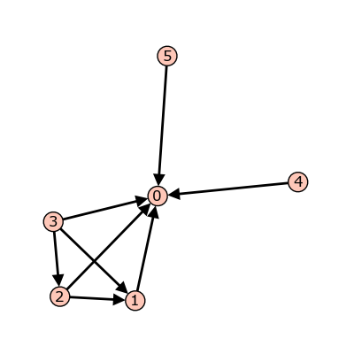
A random graph.
See sage.graphs.graph_generators for more information on the Sage graph library and graph constructors.
Each of these four formats is preprocessed by the Sandpile class so that,
internally, the graph is represented by the dictionary of dictionaries format
first presented. This internal format is returned by dict():
sage: S = Sandpile({0:[], 1:[0, 3, 4], 2:[0, 3, 5], 3: [2, 5], 4: [1, 3], 5: [2, 3]},0)
sage: S.dict()
{0: {},
 1: {0: 1, 3: 1, 4: 1},
 2: {0: 1, 3: 1, 5: 1},
 3: {2: 1, 5: 1},
 4: {1: 1, 3: 1},
 5: {2: 1, 3: 1}}
>>> from sage.all import *
>>> S = Sandpile({Integer(0):[], Integer(1):[Integer(0), Integer(3), Integer(4)], Integer(2):[Integer(0), Integer(3), Integer(5)], Integer(3): [Integer(2), Integer(5)], Integer(4): [Integer(1), Integer(3)], Integer(5): [Integer(2), Integer(3)]},Integer(0))
>>> S.dict()
{0: {},
 1: {0: 1, 3: 1, 4: 1},
 2: {0: 1, 3: 1, 5: 1},
 3: {2: 1, 5: 1},
 4: {1: 1, 3: 1},
 5: {2: 1, 3: 1}}
Note
The user is responsible for assuring that each vertex has a directed path into the designated sink. If the sink has out-edges, these will be ignored for the purposes of sandpile calculations (but not calculations on divisors).
Code for checking whether a given vertex is a sink:
sage: S = Sandpile({0:[], 1:[0, 3, 4], 2:[0, 3, 5], 3: [2, 5], 4: [1, 3], 5: [2, 3]},0)
sage: [S.distance(v,0) for v in S.vertices(sort=True)] # 0 is a sink
[0, 1, 1, 2, 2, 2]
sage: [S.distance(v,1) for v in S.vertices(sort=True)] # 1 is not a sink
[+Infinity, 0, +Infinity, +Infinity, 1, +Infinity]
>>> from sage.all import *
>>> S = Sandpile({Integer(0):[], Integer(1):[Integer(0), Integer(3), Integer(4)], Integer(2):[Integer(0), Integer(3), Integer(5)], Integer(3): [Integer(2), Integer(5)], Integer(4): [Integer(1), Integer(3)], Integer(5): [Integer(2), Integer(3)]},Integer(0))
>>> [S.distance(v,Integer(0)) for v in S.vertices(sort=True)] # 0 is a sink
[0, 1, 1, 2, 2, 2]
>>> [S.distance(v,Integer(1)) for v in S.vertices(sort=True)] # 1 is not a sink
[+Infinity, 0, +Infinity, +Infinity, 1, +Infinity]
Methods
Here are summaries of Sandpile, SandpileConfig, and SandpileDivisor
methods (functions). Each summary is followed by a list of complete
descriptions of the methods. There are many more methods available
for a Sandpile, e.g., those inherited from the class DiGraph. To see them
all, enter dir(Sandpile) or type Sandpile., including the period,
and hit TAB.
Sandpile
Summary of methods.
all_k_config — The constant configuration with all values set to k.
all_k_div — The divisor with all values set to k.
avalanche_polynomial — The avalanche polynomial.
betti — The Betti table for the homogeneous toppling ideal.
betti_complexes — The support-complexes with non-trivial homology.
burning_config — The minimal burning configuration.
burning_script — A script for the minimal burning configuration.
canonical_divisor — The canonical divisor.
dict — A dictionary of dictionaries representing a directed graph.
genus — The genus: (# non-loop edges) - (# vertices) + 1.
groebner — A Groebner basis for the homogeneous toppling ideal.
group_gens — A minimal list of generators for the sandpile group.
group_order — The size of the sandpile group.
h_vector — The number of superstable configurations in each degree.
help — List of Sandpile-specific methods (not inherited from Graph).
hilbert_function — The Hilbert function of the homogeneous toppling ideal.
ideal — The saturated homogeneous toppling ideal.
identity — The identity configuration.
in_degree — The in-degree of a vertex or a list of all in-degrees.
invariant_factors — The invariant factors of the sandpile group.
is_undirected — Is the underlying graph undirected?
jacobian_representatives — Representatives for the elements of the Jacobian group.
laplacian — The Laplacian matrix of the graph.
markov_chain — The sandpile Markov chain for configurations or divisors.
max_stable — The maximal stable configuration.
max_stable_div — The maximal stable divisor.
max_superstables — The maximal superstable configurations.
min_recurrents — The minimal recurrent elements.
nonsink_vertices — The nonsink vertices.
nonspecial_divisors — The nonspecial divisors.
out_degree — The out-degree of a vertex or a list of all out-degrees.
picard_representatives — Representatives of the divisor classes of degree d in the Picard group.
points — Generators for the multiplicative group of zeros of the sandpile ideal.
postulation — The postulation number of the toppling ideal.
recurrents — The recurrent configurations.
reduced_laplacian — The reduced Laplacian matrix of the graph.
reorder_vertices — A copy of the sandpile with vertex names permuted.
resolution — A minimal free resolution of the homogeneous toppling ideal.
ring — The ring containing the homogeneous toppling ideal.
show — Draw the underlying graph.
show3d — Draw the underlying graph.
sink — The sink vertex.
smith_form — The Smith normal form for the Laplacian.
solve — Approximations of the complex affine zeros of the sandpile ideal.
stable_configs — Generator for all stable configurations.
stationary_density — The stationary density of the sandpile.
superstables — The superstable configurations.
symmetric_recurrents — The symmetric recurrent configurations.
tutte_polynomial — The Tutte polynomial.
unsaturated_ideal — The unsaturated, homogeneous toppling ideal.
version — The version number of Sage Sandpiles.
zero_config — The all-zero configuration.
zero_div — The all-zero divisor.
Complete descriptions of Sandpile methods.
—
all_k_config(k)
The constant configuration with all values set to \(k\).
INPUT:
k– integer
OUTPUT: SandpileConfig
EXAMPLES:
sage: s = sandpiles.Diamond()
sage: s.all_k_config(7)
{1: 7, 2: 7, 3: 7}
>>> from sage.all import *
>>> s = sandpiles.Diamond()
>>> s.all_k_config(Integer(7))
{1: 7, 2: 7, 3: 7}
—
all_k_div(k)
The divisor with all values set to \(k\).
INPUT:
k– integer
OUTPUT: SandpileDivisor
EXAMPLES:
sage: S = sandpiles.House()
sage: S.all_k_div(7)
{0: 7, 1: 7, 2: 7, 3: 7, 4: 7}
>>> from sage.all import *
>>> S = sandpiles.House()
>>> S.all_k_div(Integer(7))
{0: 7, 1: 7, 2: 7, 3: 7, 4: 7}
—
avalanche_polynomial(multivariable=True)
The avalanche polynomial. See NOTE for details.
INPUT:
multivariable– (default:True) boolean
OUTPUT: polynomial
EXAMPLES:
sage: s = sandpiles.Complete(4)
sage: s.avalanche_polynomial()
9*x0*x1*x2 + 2*x0*x1 + 2*x0*x2 + 2*x1*x2 + 3*x0 + 3*x1 + 3*x2 + 24
sage: s.avalanche_polynomial(False)
9*x0^3 + 6*x0^2 + 9*x0 + 24
>>> from sage.all import *
>>> s = sandpiles.Complete(Integer(4))
>>> s.avalanche_polynomial()
9*x0*x1*x2 + 2*x0*x1 + 2*x0*x2 + 2*x1*x2 + 3*x0 + 3*x1 + 3*x2 + 24
>>> s.avalanche_polynomial(False)
9*x0^3 + 6*x0^2 + 9*x0 + 24
Note
For each nonsink vertex \(v\), let \(x_v\) be an indeterminate.
If \((r,v)\) is a pair consisting of a recurrent \(r\) and nonsink
vertex \(v\), then for each nonsink vertex \(w\), let \(n_w\) be the
number of times vertex \(w\) fires in the stabilization of \(r + v\).
Let \(M(r,v)\) be the monomial \(\prod_w x_w^{n_w}\), i.e., the exponent
records the vector of \(n_w\) as \(w\) ranges over the nonsink vertices.
The avalanche polynomial is then the sum of \(M(r,v)\) as \(r\) ranges
over the recurrents and \(v\) ranges over the nonsink vertices. If
multivariable is False, then set all the indeterminates equal
to each other (and, thus, only count the number of vertex firings in the
stabilizations, forgetting which particular vertices fired).
—
betti(verbose=True)
The Betti table for the homogeneous toppling ideal. If
verbose is True, it prints the standard Betti table, otherwise,
it returns a less formatted table.
INPUT:
verbose– (default:True) boolean
OUTPUT: Betti numbers for the sandpile
EXAMPLES:
sage: S = sandpiles.Diamond()
sage: S.betti()
           0     1     2     3
------------------------------
    0:     1     -     -     -
    1:     -     2     -     -
    2:     -     4     9     4
------------------------------
total:     1     6     9     4
sage: S.betti(False)
[1, 6, 9, 4]
>>> from sage.all import *
>>> S = sandpiles.Diamond()
>>> S.betti()
           0     1     2     3
------------------------------
    0:     1     -     -     -
    1:     -     2     -     -
    2:     -     4     9     4
------------------------------
total:     1     6     9     4
>>> S.betti(False)
[1, 6, 9, 4]
—
betti_complexes()
The support-complexes with non-trivial homology. (See NOTE.)
OUTPUT:
list (of pairs [divisors, corresponding simplicial complex])
EXAMPLES:
sage: S = Sandpile({0:{},1:{0: 1, 2: 1, 3: 4},2:{3: 5},3:{1: 1, 2: 1}},0)
sage: p = S.betti_complexes()
sage: p[0]
[{0: -8, 1: 5, 2: 4, 3: 1}, Simplicial complex with vertex set (1, 2, 3) and facets {(3,), (1, 2)}]
sage: S.resolution()
'R^1 <-- R^5 <-- R^5 <-- R^1'
sage: S.betti()
           0     1     2     3
------------------------------
    0:     1     -     -     -
    1:     -     5     5     -
    2:     -     -     -     1
------------------------------
total:     1     5     5     1
sage: len(p)
11
sage: p[0][1].homology()
{0: Z, 1: 0}
sage: p[-1][1].homology()
{0: 0, 1: 0, 2: Z}
>>> from sage.all import *
>>> S = Sandpile({Integer(0):{},Integer(1):{Integer(0): Integer(1), Integer(2): Integer(1), Integer(3): Integer(4)},Integer(2):{Integer(3): Integer(5)},Integer(3):{Integer(1): Integer(1), Integer(2): Integer(1)}},Integer(0))
>>> p = S.betti_complexes()
>>> p[Integer(0)]
[{0: -8, 1: 5, 2: 4, 3: 1}, Simplicial complex with vertex set (1, 2, 3) and facets {(3,), (1, 2)}]
>>> S.resolution()
'R^1 <-- R^5 <-- R^5 <-- R^1'
>>> S.betti()
           0     1     2     3
------------------------------
    0:     1     -     -     -
    1:     -     5     5     -
    2:     -     -     -     1
------------------------------
total:     1     5     5     1
>>> len(p)
11
>>> p[Integer(0)][Integer(1)].homology()
{0: Z, 1: 0}
>>> p[-Integer(1)][Integer(1)].homology()
{0: 0, 1: 0, 2: Z}
Note
A support-complex is the simplicial complex formed from the
supports of the divisors in a linear system.
—
burning_config()
The minimal burning configuration.
OUTPUT:
dict (configuration)
EXAMPLES:
sage: g = {0:{},1:{0:1,3:1,4:1},2:{0:1,3:1,5:1}, \
....:      3:{2:1,5:1},4:{1:1,3:1},5:{2:1,3:1}}
sage: S = Sandpile(g,0)
sage: S.burning_config()
{1: 2, 2: 0, 3: 1, 4: 1, 5: 0}
sage: S.burning_config().values()
[2, 0, 1, 1, 0]
sage: S.burning_script()
{1: 1, 2: 3, 3: 5, 4: 1, 5: 4}
sage: script = S.burning_script().values()
sage: script
[1, 3, 5, 1, 4]
sage: matrix(script)*S.reduced_laplacian()
[2 0 1 1 0]
>>> from sage.all import *
>>> g = {Integer(0):{},Integer(1):{Integer(0):Integer(1),Integer(3):Integer(1),Integer(4):Integer(1)},Integer(2):{Integer(0):Integer(1),Integer(3):Integer(1),Integer(5):Integer(1)},      Integer(3):{Integer(2):Integer(1),Integer(5):Integer(1)},Integer(4):{Integer(1):Integer(1),Integer(3):Integer(1)},Integer(5):{Integer(2):Integer(1),Integer(3):Integer(1)}}
>>> S = Sandpile(g,Integer(0))
>>> S.burning_config()
{1: 2, 2: 0, 3: 1, 4: 1, 5: 0}
>>> S.burning_config().values()
[2, 0, 1, 1, 0]
>>> S.burning_script()
{1: 1, 2: 3, 3: 5, 4: 1, 5: 4}
>>> script = S.burning_script().values()
>>> script
[1, 3, 5, 1, 4]
>>> matrix(script)*S.reduced_laplacian()
[2 0 1 1 0]
Note
The burning configuration and script are computed using a modified version of Speer’s script algorithm. This is a generalization to directed multigraphs of Dhar’s burning algorithm.
A burning configuration is a nonnegative integer-linear combination of the rows of the reduced Laplacian matrix having nonnegative entries and such that every vertex has a path from some vertex in its support. The corresponding burning script gives the integer-linear combination needed to obtain the burning configuration. So if \(b\) is the burning configuration, \(\sigma\) is its script, and \(\tilde{L}\) is the reduced Laplacian, then \(\sigma\cdot \tilde{L} = b\). The minimal burning configuration is the one with the minimal script (its components are no larger than the components of any other script for a burning configuration).
The following are equivalent for a configuration \(c\) with burning configuration \(b\) having script \(\sigma\):
\(c\) is recurrent;
\(c+b\) stabilizes to \(c\);
the firing vector for the stabilization of \(c+b\) is \(\sigma\).
—
burning_script()
A script for the minimal burning configuration.
OUTPUT: dict
EXAMPLES:
sage: g = {0:{},1:{0:1,3:1,4:1},2:{0:1,3:1,5:1},\
....: 3:{2:1,5:1},4:{1:1,3:1},5:{2:1,3:1}}
sage: S = Sandpile(g,0)
sage: S.burning_config()
{1: 2, 2: 0, 3: 1, 4: 1, 5: 0}
sage: S.burning_config().values()
[2, 0, 1, 1, 0]
sage: S.burning_script()
{1: 1, 2: 3, 3: 5, 4: 1, 5: 4}
sage: script = S.burning_script().values()
sage: script
[1, 3, 5, 1, 4]
sage: matrix(script)*S.reduced_laplacian()
[2 0 1 1 0]
>>> from sage.all import *
>>> g = {Integer(0):{},Integer(1):{Integer(0):Integer(1),Integer(3):Integer(1),Integer(4):Integer(1)},Integer(2):{Integer(0):Integer(1),Integer(3):Integer(1),Integer(5):Integer(1)},Integer(3):{Integer(2):Integer(1),Integer(5):Integer(1)},Integer(4):{Integer(1):Integer(1),Integer(3):Integer(1)},Integer(5):{Integer(2):Integer(1),Integer(3):Integer(1)}}
>>> S = Sandpile(g,Integer(0))
>>> S.burning_config()
{1: 2, 2: 0, 3: 1, 4: 1, 5: 0}
>>> S.burning_config().values()
[2, 0, 1, 1, 0]
>>> S.burning_script()
{1: 1, 2: 3, 3: 5, 4: 1, 5: 4}
>>> script = S.burning_script().values()
>>> script
[1, 3, 5, 1, 4]
>>> matrix(script)*S.reduced_laplacian()
[2 0 1 1 0]
Note
The burning configuration and script are computed using a modified version of Speer’s script algorithm. This is a generalization to directed multigraphs of Dhar’s burning algorithm.
A burning configuration is a nonnegative integer-linear combination of the rows of the reduced Laplacian matrix having nonnegative entries and such that every vertex has a path from some vertex in its support. The corresponding burning script gives the integer-linear combination needed to obtain the burning configuration. So if \(b\) is the burning configuration, \(s\) is its script, and \(L_{\mathrm{red}}\) is the reduced Laplacian, then \(s\cdot L_{\mathrm{red}}= b\). The minimal burning configuration is the one with the minimal script (its components are no larger than the components of any other script for a burning configuration).
The following are equivalent for a configuration \(c\) with burning configuration \(b\) having script \(s\):
\(c\) is recurrent;
\(c+b\) stabilizes to \(c\);
the firing vector for the stabilization of \(c+b\) is \(s\).
—
canonical_divisor()
The canonical divisor. This is the divisor with \(\deg(v)-2\) grains of sand on each vertex (not counting loops). Only for undirected graphs.
OUTPUT: SandpileDivisor
EXAMPLES:
sage: S = sandpiles.Complete(4)
sage: S.canonical_divisor()
{0: 1, 1: 1, 2: 1, 3: 1}
sage: s = Sandpile({0:[1,1],1:[0,0,1,1,1]},0)
sage: s.canonical_divisor()  # loops are disregarded
{0: 0, 1: 0}
>>> from sage.all import *
>>> S = sandpiles.Complete(Integer(4))
>>> S.canonical_divisor()
{0: 1, 1: 1, 2: 1, 3: 1}
>>> s = Sandpile({Integer(0):[Integer(1),Integer(1)],Integer(1):[Integer(0),Integer(0),Integer(1),Integer(1),Integer(1)]},Integer(0))
>>> s.canonical_divisor()  # loops are disregarded
{0: 0, 1: 0}
Warning
The underlying graph must be undirected.
—
dict()
A dictionary of dictionaries representing a directed graph.
OUTPUT: dict
EXAMPLES:
sage: S = sandpiles.Diamond()
sage: S.dict()
{0: {1: 1, 2: 1},
 1: {0: 1, 2: 1, 3: 1},
 2: {0: 1, 1: 1, 3: 1},
 3: {1: 1, 2: 1}}
sage: S.sink()
0
>>> from sage.all import *
>>> S = sandpiles.Diamond()
>>> S.dict()
{0: {1: 1, 2: 1},
 1: {0: 1, 2: 1, 3: 1},
 2: {0: 1, 1: 1, 3: 1},
 3: {1: 1, 2: 1}}
>>> S.sink()
0
—
genus()
The genus: (# non-loop edges) - (# vertices) + 1. Only defined for undirected graphs.
OUTPUT: integer
EXAMPLES:
sage: sandpiles.Complete(4).genus()
3
sage: sandpiles.Cycle(5).genus()
1
>>> from sage.all import *
>>> sandpiles.Complete(Integer(4)).genus()
3
>>> sandpiles.Cycle(Integer(5)).genus()
1
—
groebner()
A Groebner basis for the homogeneous toppling ideal. It is computed
with respect to the standard sandpile ordering (see ring).
OUTPUT: Groebner basis
EXAMPLES:
sage: S = sandpiles.Diamond()
sage: S.groebner()
[x3*x2^2 - x1^2*x0, x2^3 - x3*x1*x0, x3*x1^2 - x2^2*x0, x1^3 - x3*x2*x0, x3^2 - x0^2, x2*x1 - x0^2]
>>> from sage.all import *
>>> S = sandpiles.Diamond()
>>> S.groebner()
[x3*x2^2 - x1^2*x0, x2^3 - x3*x1*x0, x3*x1^2 - x2^2*x0, x1^3 - x3*x2*x0, x3^2 - x0^2, x2*x1 - x0^2]
—
group_gens(verbose=True)
A minimal list of generators for the sandpile group. If verbose is False
then the generators are represented as lists of integers.
INPUT:
verbose– (default:True) boolean
OUTPUT:
list of SandpileConfig (or of lists of integers if verbose is False)
EXAMPLES:
sage: s = sandpiles.Cycle(5)
sage: s.group_gens()
[{1: 0, 2: 1, 3: 1, 4: 1}]
sage: s.group_gens()[0].order()
5
sage: s = sandpiles.Complete(5)
sage: s.group_gens(False)
[[2, 3, 2, 2], [2, 2, 3, 2], [2, 2, 2, 3]]
sage: [i.order() for i in s.group_gens()]
[5, 5, 5]
sage: s.invariant_factors()
[1, 5, 5, 5]
>>> from sage.all import *
>>> s = sandpiles.Cycle(Integer(5))
>>> s.group_gens()
[{1: 0, 2: 1, 3: 1, 4: 1}]
>>> s.group_gens()[Integer(0)].order()
5
>>> s = sandpiles.Complete(Integer(5))
>>> s.group_gens(False)
[[2, 3, 2, 2], [2, 2, 3, 2], [2, 2, 2, 3]]
>>> [i.order() for i in s.group_gens()]
[5, 5, 5]
>>> s.invariant_factors()
[1, 5, 5, 5]
—
group_order()
The size of the sandpile group.
OUTPUT: integer
EXAMPLES:
sage: S = sandpiles.House()
sage: S.group_order()
11
>>> from sage.all import *
>>> S = sandpiles.House()
>>> S.group_order()
11
—
h_vector()
The number of superstable configurations in each degree. Equivalently, this is the list of first differences of the Hilbert function of the (homogeneous) toppling ideal.
OUTPUT: list of nonnegative integers
EXAMPLES:
sage: s = sandpiles.Grid(2,2)
sage: s.hilbert_function()
[1, 5, 15, 35, 66, 106, 146, 178, 192]
sage: s.h_vector()
[1, 4, 10, 20, 31, 40, 40, 32, 14]
>>> from sage.all import *
>>> s = sandpiles.Grid(Integer(2),Integer(2))
>>> s.hilbert_function()
[1, 5, 15, 35, 66, 106, 146, 178, 192]
>>> s.h_vector()
[1, 4, 10, 20, 31, 40, 40, 32, 14]
—
help(verbose=True)
List of Sandpile-specific methods (not inherited from Graph). If verbose, include short descriptions.
INPUT:
verbose– (default:True) boolean
OUTPUT: printed string
EXAMPLES:
sage: Sandpile.help()
For detailed help with any method FOO listed below,
enter "Sandpile.FOO?" or enter "S.FOO?" for any Sandpile S.

all_k_config             -- The constant configuration with all values set to k.
all_k_div                -- The divisor with all values set to k.
avalanche_polynomial     -- The avalanche polynomial.
betti                    -- The Betti table for the homogeneous toppling ideal.
betti_complexes          -- The support-complexes with non-trivial homology.
...
unsaturated_ideal        -- The unsaturated, homogeneous toppling ideal.
version                  -- The version number of Sage Sandpiles.
zero_config              -- The all-zero configuration.
zero_div                 -- The all-zero divisor.
>>> from sage.all import *
>>> Sandpile.help()
For detailed help with any method FOO listed below,
enter "Sandpile.FOO?" or enter "S.FOO?" for any Sandpile S.
<BLANKLINE>
all_k_config             -- The constant configuration with all values set to k.
all_k_div                -- The divisor with all values set to k.
avalanche_polynomial     -- The avalanche polynomial.
betti                    -- The Betti table for the homogeneous toppling ideal.
betti_complexes          -- The support-complexes with non-trivial homology.
...
unsaturated_ideal        -- The unsaturated, homogeneous toppling ideal.
version                  -- The version number of Sage Sandpiles.
zero_config              -- The all-zero configuration.
zero_div                 -- The all-zero divisor.
—
hilbert_function()
The Hilbert function of the homogeneous toppling ideal.
OUTPUT: list of nonnegative integers
EXAMPLES:
sage: s = sandpiles.Wheel(5)
sage: s.hilbert_function()
[1, 5, 15, 31, 45]
sage: s.h_vector()
[1, 4, 10, 16, 14]
>>> from sage.all import *
>>> s = sandpiles.Wheel(Integer(5))
>>> s.hilbert_function()
[1, 5, 15, 31, 45]
>>> s.h_vector()
[1, 4, 10, 16, 14]
—
ideal(gens=False)
The saturated homogeneous toppling ideal. If gens is True, the
generators for the ideal are returned instead.
INPUT:
gens– (default:False) boolean
OUTPUT: ideal or, optionally, the generators of an ideal
EXAMPLES:
sage: S = sandpiles.Diamond()
sage: S.ideal()
Ideal (x2*x1 - x0^2, x3^2 - x0^2, x1^3 - x3*x2*x0, x3*x1^2 - x2^2*x0, x2^3 - x3*x1*x0, x3*x2^2 - x1^2*x0) of Multivariate Polynomial Ring in x3, x2, x1, x0 over Rational Field
sage: S.ideal(True)
[x2*x1 - x0^2, x3^2 - x0^2, x1^3 - x3*x2*x0, x3*x1^2 - x2^2*x0, x2^3 - x3*x1*x0, x3*x2^2 - x1^2*x0]
sage: S.ideal().gens()  # another way to get the generators
[x2*x1 - x0^2, x3^2 - x0^2, x1^3 - x3*x2*x0, x3*x1^2 - x2^2*x0, x2^3 - x3*x1*x0, x3*x2^2 - x1^2*x0]
>>> from sage.all import *
>>> S = sandpiles.Diamond()
>>> S.ideal()
Ideal (x2*x1 - x0^2, x3^2 - x0^2, x1^3 - x3*x2*x0, x3*x1^2 - x2^2*x0, x2^3 - x3*x1*x0, x3*x2^2 - x1^2*x0) of Multivariate Polynomial Ring in x3, x2, x1, x0 over Rational Field
>>> S.ideal(True)
[x2*x1 - x0^2, x3^2 - x0^2, x1^3 - x3*x2*x0, x3*x1^2 - x2^2*x0, x2^3 - x3*x1*x0, x3*x2^2 - x1^2*x0]
>>> S.ideal().gens()  # another way to get the generators
[x2*x1 - x0^2, x3^2 - x0^2, x1^3 - x3*x2*x0, x3*x1^2 - x2^2*x0, x2^3 - x3*x1*x0, x3*x2^2 - x1^2*x0]
—
identity(verbose=True)
The identity configuration. If verbose is False, the
configuration are converted to a list of integers.
INPUT:
verbose– (default:True) boolean
OUTPUT:
SandpileConfig or a list of integers If verbose is False, the
configuration are converted to a list of integers.
EXAMPLES:
sage: s = sandpiles.Diamond()
sage: s.identity()
{1: 2, 2: 2, 3: 0}
sage: s.identity(False)
[2, 2, 0]
sage: s.identity() & s.max_stable() == s.max_stable()
True
>>> from sage.all import *
>>> s = sandpiles.Diamond()
>>> s.identity()
{1: 2, 2: 2, 3: 0}
>>> s.identity(False)
[2, 2, 0]
>>> s.identity() & s.max_stable() == s.max_stable()
True
—
in_degree(v=None)
The in-degree of a vertex or a list of all in-degrees.
INPUT:
v– (optional) vertex name
OUTPUT: integer or dict
EXAMPLES:
sage: s = sandpiles.House()
sage: s.in_degree()
{0: 2, 1: 2, 2: 3, 3: 3, 4: 2}
sage: s.in_degree(2)
3
>>> from sage.all import *
>>> s = sandpiles.House()
>>> s.in_degree()
{0: 2, 1: 2, 2: 3, 3: 3, 4: 2}
>>> s.in_degree(Integer(2))
3
—
invariant_factors()
The invariant factors of the sandpile group.
OUTPUT: list of integers
EXAMPLES:
sage: s = sandpiles.Grid(2,2)
sage: s.invariant_factors()
[1, 1, 8, 24]
>>> from sage.all import *
>>> s = sandpiles.Grid(Integer(2),Integer(2))
>>> s.invariant_factors()
[1, 1, 8, 24]
—
is_undirected()
Is the underlying graph undirected? True if \((u,v)\) is and edge if
and only if \((v,u)\) is an edge, each edge with the same weight.
OUTPUT: boolean
EXAMPLES:
sage: sandpiles.Complete(4).is_undirected()
True
sage: s = Sandpile({0:[1,2], 1:[0,2], 2:[0]}, 0)
sage: s.is_undirected()
False
>>> from sage.all import *
>>> sandpiles.Complete(Integer(4)).is_undirected()
True
>>> s = Sandpile({Integer(0):[Integer(1),Integer(2)], Integer(1):[Integer(0),Integer(2)], Integer(2):[Integer(0)]}, Integer(0))
>>> s.is_undirected()
False
—
jacobian_representatives(verbose=True)
Representatives for the elements of the Jacobian group. If verbose
is False, then lists representing the divisors are returned.
INPUT:
verbose– (default:True) boolean
OUTPUT:
list of SandpileDivisor (or of lists representing divisors)
EXAMPLES:
For an undirected graph, divisors of the form s - deg(s)*sink as
s varies over the superstables forms a distinct set of
representatives for the Jacobian group.:
sage: s = sandpiles.Complete(3)
sage: s.superstables(False)
[[0, 0], [0, 1], [1, 0]]
sage: s.jacobian_representatives(False)
[[0, 0, 0], [-1, 0, 1], [-1, 1, 0]]
>>> from sage.all import *
>>> s = sandpiles.Complete(Integer(3))
>>> s.superstables(False)
[[0, 0], [0, 1], [1, 0]]
>>> s.jacobian_representatives(False)
[[0, 0, 0], [-1, 0, 1], [-1, 1, 0]]
If the graph is directed, the representatives described above may by equivalent modulo the rowspan of the Laplacian matrix:
sage: s = Sandpile({0: {1: 1, 2: 2}, 1: {0: 2, 2: 4}, 2: {0: 4, 1: 2}},0)
sage: s.group_order()
28
sage: s.jacobian_representatives()
[{0: -5, 1: 3, 2: 2}, {0: -4, 1: 3, 2: 1}]
>>> from sage.all import *
>>> s = Sandpile({Integer(0): {Integer(1): Integer(1), Integer(2): Integer(2)}, Integer(1): {Integer(0): Integer(2), Integer(2): Integer(4)}, Integer(2): {Integer(0): Integer(4), Integer(1): Integer(2)}},Integer(0))
>>> s.group_order()
28
>>> s.jacobian_representatives()
[{0: -5, 1: 3, 2: 2}, {0: -4, 1: 3, 2: 1}]
Let \(\tau\) be the nonnegative generator of the kernel of the transpose of the Laplacian, and let \(tau_s\) be it sink component, then the sandpile group is isomorphic to the direct sum of the cyclic group of order \(\tau_s\) and the Jacobian group. In the example above, we have:
sage: s.laplacian().left_kernel()
Free module of degree 3 and rank 1 over Integer Ring
Echelon basis matrix:
[14  5  8]
>>> from sage.all import *
>>> s.laplacian().left_kernel()
Free module of degree 3 and rank 1 over Integer Ring
Echelon basis matrix:
[14  5  8]
Note
The Jacobian group is the set of all divisors of degree zero modulo the integer rowspan of the Laplacian matrix.
—
laplacian()
The Laplacian matrix of the graph. Its rows encode the vertex firing rules.
OUTPUT: matrix
EXAMPLES:
sage: G = sandpiles.Diamond()
sage: G.laplacian()
[ 2 -1 -1  0]
[-1  3 -1 -1]
[-1 -1  3 -1]
[ 0 -1 -1  2]
>>> from sage.all import *
>>> G = sandpiles.Diamond()
>>> G.laplacian()
[ 2 -1 -1  0]
[-1  3 -1 -1]
[-1 -1  3 -1]
[ 0 -1 -1  2]
Warning
The function laplacian_matrix should be avoided. It returns the
indegree version of the Laplacian.
—
markov_chain(state, distrib=None)
The sandpile Markov chain for configurations or divisors.
The chain starts at state. See NOTE for details.
INPUT:
state– SandpileConfig, SandpileDivisor, or list representing one of thesedistrib– (optional) list of nonnegative numbers summing to 1 (representing a prob. dist.)
OUTPUT:
generator for Markov chain (see NOTE)
EXAMPLES:
sage: s = sandpiles.Complete(4)
sage: m = s.markov_chain([0,0,0])
sage: next(m)          # random
{1: 0, 2: 0, 3: 0}
sage: next(m).values() # random
[0, 0, 0]
sage: next(m).values() # random
[0, 0, 0]
sage: next(m).values() # random
[0, 0, 0]
sage: next(m).values() # random
[0, 1, 0]
sage: next(m).values() # random
[0, 2, 0]
sage: next(m).values() # random
[0, 2, 1]
sage: next(m).values() # random
[1, 2, 1]
sage: next(m).values() # random
[2, 2, 1]
sage: m = s.markov_chain(s.zero_div(), [0.1,0.1,0.1,0.7])
sage: next(m).values() # random
[0, 0, 0, 1]
sage: next(m).values() # random
[0, 0, 1, 1]
sage: next(m).values() # random
[0, 0, 1, 2]
sage: next(m).values() # random
[1, 1, 2, 0]
sage: next(m).values() # random
[1, 1, 2, 1]
sage: next(m).values() # random
[1, 1, 2, 2]
sage: next(m).values() # random
[1, 1, 2, 3]
sage: next(m).values() # random
[1, 1, 2, 4]
sage: next(m).values() # random
[1, 1, 3, 4]
>>> from sage.all import *
>>> s = sandpiles.Complete(Integer(4))
>>> m = s.markov_chain([Integer(0),Integer(0),Integer(0)])
>>> next(m)          # random
{1: 0, 2: 0, 3: 0}
>>> next(m).values() # random
[0, 0, 0]
>>> next(m).values() # random
[0, 0, 0]
>>> next(m).values() # random
[0, 0, 0]
>>> next(m).values() # random
[0, 1, 0]
>>> next(m).values() # random
[0, 2, 0]
>>> next(m).values() # random
[0, 2, 1]
>>> next(m).values() # random
[1, 2, 1]
>>> next(m).values() # random
[2, 2, 1]
>>> m = s.markov_chain(s.zero_div(), [RealNumber('0.1'),RealNumber('0.1'),RealNumber('0.1'),RealNumber('0.7')])
>>> next(m).values() # random
[0, 0, 0, 1]
>>> next(m).values() # random
[0, 0, 1, 1]
>>> next(m).values() # random
[0, 0, 1, 2]
>>> next(m).values() # random
[1, 1, 2, 0]
>>> next(m).values() # random
[1, 1, 2, 1]
>>> next(m).values() # random
[1, 1, 2, 2]
>>> next(m).values() # random
[1, 1, 2, 3]
>>> next(m).values() # random
[1, 1, 2, 4]
>>> next(m).values() # random
[1, 1, 3, 4]
Note
The closed sandpile Markov chain has state space consisting of the configurations
on a sandpile. It transitions from a state by choosing a vertex at random
(according to the probability distribution distrib), dropping a grain of sand at
that vertex, and stabilizing. If the chosen vertex is the sink, the chain stays
at the current state.
The open sandpile Markov chain has state space consisting of the recurrent elements,
i.e., the state space is the sandpile group. It transitions from the configuration \(c\)
by choosing a vertex \(v\) at random according to distrib. The next state is the
stabilization of \(c+v\). If \(v\) is the sink vertex, then the stabilization of \(c+v\)
is defined to be \(c\).
Note that in either case, if distrib is specified, its length is equal to
the total number of vertices (including the sink).
REFERENCES:
Lionel Levine. Threshold state and a conjecture of Poghosyan, Poghosyan, Priezzhev and Ruelle, Communications in Mathematical Physics. arXiv 1402.3283
—
max_stable()
The maximal stable configuration.
OUTPUT:
SandpileConfig (the maximal stable configuration)
EXAMPLES:
sage: S = sandpiles.House()
sage: S.max_stable()
{1: 1, 2: 2, 3: 2, 4: 1}
>>> from sage.all import *
>>> S = sandpiles.House()
>>> S.max_stable()
{1: 1, 2: 2, 3: 2, 4: 1}
—
max_stable_div()
The maximal stable divisor.
OUTPUT:
SandpileDivisor (the maximal stable divisor)
EXAMPLES:
sage: s = sandpiles.Diamond()
sage: s.max_stable_div()
{0: 1, 1: 2, 2: 2, 3: 1}
sage: s.out_degree()
{0: 2, 1: 3, 2: 3, 3: 2}
>>> from sage.all import *
>>> s = sandpiles.Diamond()
>>> s.max_stable_div()
{0: 1, 1: 2, 2: 2, 3: 1}
>>> s.out_degree()
{0: 2, 1: 3, 2: 3, 3: 2}
—
max_superstables(verbose=True)
The maximal superstable configurations. If the underlying graph is
undirected, these are the superstables of highest degree. If
verbose is False, the configurations are converted to lists of
integers.
INPUT:
verbose– (default:True) boolean
OUTPUT: tuple of SandpileConfig
EXAMPLES:
sage: s = sandpiles.Diamond()
sage: s.superstables(False)
[[0, 0, 0],
 [0, 0, 1],
 [1, 0, 1],
 [0, 2, 0],
 [2, 0, 0],
 [0, 1, 1],
 [1, 0, 0],
 [0, 1, 0]]
sage: s.max_superstables(False)
[[1, 0, 1], [0, 2, 0], [2, 0, 0], [0, 1, 1]]
sage: s.h_vector()
[1, 3, 4]
>>> from sage.all import *
>>> s = sandpiles.Diamond()
>>> s.superstables(False)
[[0, 0, 0],
 [0, 0, 1],
 [1, 0, 1],
 [0, 2, 0],
 [2, 0, 0],
 [0, 1, 1],
 [1, 0, 0],
 [0, 1, 0]]
>>> s.max_superstables(False)
[[1, 0, 1], [0, 2, 0], [2, 0, 0], [0, 1, 1]]
>>> s.h_vector()
[1, 3, 4]
—
min_recurrents(verbose=True)
The minimal recurrent elements. If the underlying graph is
undirected, these are the recurrent elements of least degree.
If verbose is False, the configurations are converted
to lists of integers.
INPUT:
verbose– (default:True) boolean
OUTPUT: list of SandpileConfig
EXAMPLES:
sage: s = sandpiles.Diamond()
sage: s.recurrents(False)
[[2, 2, 1],
 [2, 2, 0],
 [1, 2, 0],
 [2, 0, 1],
 [0, 2, 1],
 [2, 1, 0],
 [1, 2, 1],
 [2, 1, 1]]
sage: s.min_recurrents(False)
[[1, 2, 0], [2, 0, 1], [0, 2, 1], [2, 1, 0]]
sage: [i.deg() for i in s.recurrents()]
[5, 4, 3, 3, 3, 3, 4, 4]
>>> from sage.all import *
>>> s = sandpiles.Diamond()
>>> s.recurrents(False)
[[2, 2, 1],
 [2, 2, 0],
 [1, 2, 0],
 [2, 0, 1],
 [0, 2, 1],
 [2, 1, 0],
 [1, 2, 1],
 [2, 1, 1]]
>>> s.min_recurrents(False)
[[1, 2, 0], [2, 0, 1], [0, 2, 1], [2, 1, 0]]
>>> [i.deg() for i in s.recurrents()]
[5, 4, 3, 3, 3, 3, 4, 4]
—
nonsink_vertices()
The nonsink vertices.
OUTPUT: list of vertices
EXAMPLES:
sage: s = sandpiles.Grid(2,3)
sage: s.nonsink_vertices()
[(1, 1), (1, 2), (1, 3), (2, 1), (2, 2), (2, 3)]
>>> from sage.all import *
>>> s = sandpiles.Grid(Integer(2),Integer(3))
>>> s.nonsink_vertices()
[(1, 1), (1, 2), (1, 3), (2, 1), (2, 2), (2, 3)]
—
nonspecial_divisors(verbose=True)
The nonspecial divisors. Only for undirected graphs. (See NOTE.)
INPUT:
verbose– (default:True) boolean
OUTPUT:
list (of divisors)
EXAMPLES:
sage: S = sandpiles.Complete(4)
sage: ns = S.nonspecial_divisors()
sage: D = ns[0]
sage: D.values()
[-1, 0, 1, 2]
sage: D.deg()
2
sage: [i.effective_div() for i in ns]
[[], [], [], [], [], []]
>>> from sage.all import *
>>> S = sandpiles.Complete(Integer(4))
>>> ns = S.nonspecial_divisors()
>>> D = ns[Integer(0)]
>>> D.values()
[-1, 0, 1, 2]
>>> D.deg()
2
>>> [i.effective_div() for i in ns]
[[], [], [], [], [], []]
Note
The “nonspecial divisors” are those divisors of degree \(g-1\) with
empty linear system. The term is only defined for undirected graphs.
Here, \(g = |E| - |V| + 1\) is the genus of the graph (not counting loops
as part of \(|E|\)). If verbose is False, the divisors are converted
to lists of integers.
Warning
The underlying graph must be undirected.
—
out_degree(v=None)
The out-degree of a vertex or a list of all out-degrees.
INPUT:
v- (optional) vertex name
OUTPUT: integer or dict
EXAMPLES:
sage: s = sandpiles.House()
sage: s.out_degree()
{0: 2, 1: 2, 2: 3, 3: 3, 4: 2}
sage: s.out_degree(2)
3
>>> from sage.all import *
>>> s = sandpiles.House()
>>> s.out_degree()
{0: 2, 1: 2, 2: 3, 3: 3, 4: 2}
>>> s.out_degree(Integer(2))
3
—
picard_representatives(d, verbose=True)
Representatives of the divisor classes of degree \(d\) in the Picard group. (Also
see the documentation for jacobian_representatives.)
INPUT:
d– integerverbose– (default:True) boolean
OUTPUT:
list of SandpileDivisors (or lists representing divisors)
EXAMPLES:
sage: s = sandpiles.Complete(3)
sage: s.superstables(False)
[[0, 0], [0, 1], [1, 0]]
sage: s.jacobian_representatives(False)
[[0, 0, 0], [-1, 0, 1], [-1, 1, 0]]
sage: s.picard_representatives(3,False)
[[3, 0, 0], [2, 0, 1], [2, 1, 0]]
>>> from sage.all import *
>>> s = sandpiles.Complete(Integer(3))
>>> s.superstables(False)
[[0, 0], [0, 1], [1, 0]]
>>> s.jacobian_representatives(False)
[[0, 0, 0], [-1, 0, 1], [-1, 1, 0]]
>>> s.picard_representatives(Integer(3),False)
[[3, 0, 0], [2, 0, 1], [2, 1, 0]]
—
points()
Generators for the multiplicative group of zeros of the sandpile ideal.
OUTPUT: list of complex numbers
EXAMPLES:
The sandpile group in this example is cyclic, and hence there is a single generator for the group of solutions.
sage: S = sandpiles.Complete(4)
sage: S.points()
[[-I, I, 1], [-I, 1, I]]
>>> from sage.all import *
>>> S = sandpiles.Complete(Integer(4))
>>> S.points()
[[-I, I, 1], [-I, 1, I]]
—
postulation()
The postulation number of the toppling ideal. This is the largest weight of a superstable configuration of the graph.
OUTPUT: nonnegative integer
EXAMPLES:
sage: s = sandpiles.Complete(4)
sage: s.postulation()
3
>>> from sage.all import *
>>> s = sandpiles.Complete(Integer(4))
>>> s.postulation()
3
—
recurrents(verbose=True)
The recurrent configurations. If verbose is False, the
configurations are converted to lists of integers.
INPUT:
verbose– (default:True) boolean
OUTPUT: list of recurrent configurations
EXAMPLES:
sage: r = Sandpile(graphs.HouseXGraph(),0).recurrents()
sage: r[:3]
[{1: 2, 2: 3, 3: 3, 4: 1}, {1: 1, 2: 3, 3: 3, 4: 0}, {1: 1, 2: 3, 3: 3, 4: 1}]
sage: sandpiles.Complete(4).recurrents(False)
[[2, 2, 2],
 [2, 2, 1],
 [2, 1, 2],
 [1, 2, 2],
 [2, 2, 0],
 [2, 0, 2],
 [0, 2, 2],
 [2, 1, 1],
 [1, 2, 1],
 [1, 1, 2],
 [2, 1, 0],
 [2, 0, 1],
 [1, 2, 0],
 [1, 0, 2],
 [0, 2, 1],
 [0, 1, 2]]
sage: sandpiles.Cycle(4).recurrents(False)
[[1, 1, 1], [0, 1, 1], [1, 0, 1], [1, 1, 0]]
>>> from sage.all import *
>>> r = Sandpile(graphs.HouseXGraph(),Integer(0)).recurrents()
>>> r[:Integer(3)]
[{1: 2, 2: 3, 3: 3, 4: 1}, {1: 1, 2: 3, 3: 3, 4: 0}, {1: 1, 2: 3, 3: 3, 4: 1}]
>>> sandpiles.Complete(Integer(4)).recurrents(False)
[[2, 2, 2],
 [2, 2, 1],
 [2, 1, 2],
 [1, 2, 2],
 [2, 2, 0],
 [2, 0, 2],
 [0, 2, 2],
 [2, 1, 1],
 [1, 2, 1],
 [1, 1, 2],
 [2, 1, 0],
 [2, 0, 1],
 [1, 2, 0],
 [1, 0, 2],
 [0, 2, 1],
 [0, 1, 2]]
>>> sandpiles.Cycle(Integer(4)).recurrents(False)
[[1, 1, 1], [0, 1, 1], [1, 0, 1], [1, 1, 0]]
—
reduced_laplacian()
The reduced Laplacian matrix of the graph.
OUTPUT: matrix
EXAMPLES:
sage: S = sandpiles.Diamond()
sage: S.laplacian()
[ 2 -1 -1  0]
[-1  3 -1 -1]
[-1 -1  3 -1]
[ 0 -1 -1  2]
sage: S.reduced_laplacian()
[ 3 -1 -1]
[-1  3 -1]
[-1 -1  2]
>>> from sage.all import *
>>> S = sandpiles.Diamond()
>>> S.laplacian()
[ 2 -1 -1  0]
[-1  3 -1 -1]
[-1 -1  3 -1]
[ 0 -1 -1  2]
>>> S.reduced_laplacian()
[ 3 -1 -1]
[-1  3 -1]
[-1 -1  2]
Note
This is the Laplacian matrix with the row and column indexed by the sink vertex removed.
—
reorder_vertices()
A copy of the sandpile with vertex names permuted. After reordering, vertex \(u\) comes before vertex \(v\) in the list of vertices if \(u\) is closer to the sink.
OUTPUT: Sandpile
EXAMPLES:
sage: S = Sandpile({0:[1], 2:[0,1], 1:[2]})
sage: S.dict()
{0: {1: 1}, 1: {2: 1}, 2: {0: 1, 1: 1}}
sage: T = S.reorder_vertices()
>>> from sage.all import *
>>> S = Sandpile({Integer(0):[Integer(1)], Integer(2):[Integer(0),Integer(1)], Integer(1):[Integer(2)]})
>>> S.dict()
{0: {1: 1}, 1: {2: 1}, 2: {0: 1, 1: 1}}
>>> T = S.reorder_vertices()
The vertices 1 and 2 have been swapped:
sage: T.dict()
{0: {1: 1}, 1: {0: 1, 2: 1}, 2: {0: 1}}
>>> from sage.all import *
>>> T.dict()
{0: {1: 1}, 1: {0: 1, 2: 1}, 2: {0: 1}}
—
resolution(verbose=False)
A minimal free resolution of the homogeneous toppling ideal. If
verbose is True, then all of the mappings are returned.
Otherwise, the resolution is summarized.
INPUT:
verbose– (default:False) boolean
OUTPUT: free resolution of the toppling ideal
EXAMPLES:
sage: S = Sandpile({0: {}, 1: {0: 1, 2: 1, 3: 4}, 2: {3: 5}, 3: {1: 1, 2: 1}},0)
sage: S.resolution()  # a Gorenstein sandpile graph
'R^1 <-- R^5 <-- R^5 <-- R^1'
sage: S.resolution(True)
[
[ x1^2 - x3*x0 x3*x1 - x2*x0  x3^2 - x2*x1  x2*x3 - x0^2  x2^2 - x1*x0],

[ x3  x2   0  x0   0]  [ x2^2 - x1*x0]
[-x1 -x3  x2   0 -x0]  [-x2*x3 + x0^2]
[ x0  x1   0  x2   0]  [-x3^2 + x2*x1]
[  0   0 -x1 -x3  x2]  [x3*x1 - x2*x0]
[  0   0  x0  x1 -x3], [ x1^2 - x3*x0]
]
sage: r = S.resolution(True)
sage: r[0]*r[1]
[0 0 0 0 0]
sage: r[1]*r[2]
[0]
[0]
[0]
[0]
[0]
>>> from sage.all import *
>>> S = Sandpile({Integer(0): {}, Integer(1): {Integer(0): Integer(1), Integer(2): Integer(1), Integer(3): Integer(4)}, Integer(2): {Integer(3): Integer(5)}, Integer(3): {Integer(1): Integer(1), Integer(2): Integer(1)}},Integer(0))
>>> S.resolution()  # a Gorenstein sandpile graph
'R^1 <-- R^5 <-- R^5 <-- R^1'
>>> S.resolution(True)
[
[ x1^2 - x3*x0 x3*x1 - x2*x0  x3^2 - x2*x1  x2*x3 - x0^2  x2^2 - x1*x0],
<BLANKLINE>
[ x3  x2   0  x0   0]  [ x2^2 - x1*x0]
[-x1 -x3  x2   0 -x0]  [-x2*x3 + x0^2]
[ x0  x1   0  x2   0]  [-x3^2 + x2*x1]
[  0   0 -x1 -x3  x2]  [x3*x1 - x2*x0]
[  0   0  x0  x1 -x3], [ x1^2 - x3*x0]
]
>>> r = S.resolution(True)
>>> r[Integer(0)]*r[Integer(1)]
[0 0 0 0 0]
>>> r[Integer(1)]*r[Integer(2)]
[0]
[0]
[0]
[0]
[0]
—
ring()
The ring containing the homogeneous toppling ideal.
OUTPUT: ring
EXAMPLES:
sage: S = sandpiles.Diamond()
sage: S.ring()
Multivariate Polynomial Ring in x3, x2, x1, x0 over Rational Field
sage: S.ring().gens()
(x3, x2, x1, x0)
>>> from sage.all import *
>>> S = sandpiles.Diamond()
>>> S.ring()
Multivariate Polynomial Ring in x3, x2, x1, x0 over Rational Field
>>> S.ring().gens()
(x3, x2, x1, x0)
Note
The indeterminate xi corresponds to the \(i\)-th vertex as listed my
the method vertices. The term-ordering is degrevlex with
indeterminates ordered according to their distance from the sink (larger
indeterminates are further from the sink).
—
show(**kwds)
Draw the underlying graph.
INPUT:
kwds– (optional) arguments passed to the show method for Graph or DiGraph
EXAMPLES:
sage: S = Sandpile({0:[], 1:[0,3,4], 2:[0,3,5], 3:[2,5], 4:[1,1], 5:[2,4]})
sage: S.show()
sage: S.show(graph_border=True, edge_labels=True)
>>> from sage.all import *
>>> S = Sandpile({Integer(0):[], Integer(1):[Integer(0),Integer(3),Integer(4)], Integer(2):[Integer(0),Integer(3),Integer(5)], Integer(3):[Integer(2),Integer(5)], Integer(4):[Integer(1),Integer(1)], Integer(5):[Integer(2),Integer(4)]})
>>> S.show()
>>> S.show(graph_border=True, edge_labels=True)
—
show3d(**kwds)
Draw the underlying graph.
INPUT:
kwds– (optional) arguments passed to the show method for Graph or DiGraph
EXAMPLES:
sage: S = sandpiles.House()
sage: S.show3d()
>>> from sage.all import *
>>> S = sandpiles.House()
>>> S.show3d()
—
sink()
The sink vertex.
OUTPUT: sink vertex
EXAMPLES:
sage: G = sandpiles.House()
sage: G.sink()
0
sage: H = sandpiles.Grid(2,2)
sage: H.sink()
(0, 0)
sage: type(H.sink())
<... 'tuple'>
>>> from sage.all import *
>>> G = sandpiles.House()
>>> G.sink()
0
>>> H = sandpiles.Grid(Integer(2),Integer(2))
>>> H.sink()
(0, 0)
>>> type(H.sink())
<... 'tuple'>
—
smith_form()
The Smith normal form for the Laplacian. In detail: a list of integer matrices \(D, U, V\) such that \(ULV = D\) where \(L\) is the transpose of the Laplacian, \(D\) is diagonal, and \(U\) and \(V\) are invertible over the integers.
OUTPUT: list of integer matrices
EXAMPLES:
sage: s = sandpiles.Complete(4)
sage: D,U,V = s.smith_form()
sage: D
[1 0 0 0]
[0 4 0 0]
[0 0 4 0]
[0 0 0 0]
sage: U*s.laplacian()*V == D  # laplacian symmetric => transpose not necessary
True
>>> from sage.all import *
>>> s = sandpiles.Complete(Integer(4))
>>> D,U,V = s.smith_form()
>>> D
[1 0 0 0]
[0 4 0 0]
[0 0 4 0]
[0 0 0 0]
>>> U*s.laplacian()*V == D  # laplacian symmetric => transpose not necessary
True
—
solve()
Approximations of the complex affine zeros of the sandpile ideal.
OUTPUT: list of complex numbers
EXAMPLES:
sage: S = Sandpile({0: {}, 1: {2: 2}, 2: {0: 4, 1: 1}}, 0)
sage: S.solve()
[[-0.707107000000000 + 0.707107000000000*I,
  0.707107000000000 - 0.707107000000000*I],
 [-0.707107000000000 - 0.707107000000000*I,
  0.707107000000000 + 0.707107000000000*I],
 [-I, -I],
 [I, I],
 [0.707107000000000 + 0.707107000000000*I,
  -0.707107000000000 - 0.707107000000000*I],
 [0.707107000000000 - 0.707107000000000*I,
  -0.707107000000000 + 0.707107000000000*I],
 [1, 1],
 [-1, -1]]
sage: len(_)
8
sage: S.group_order()
8
>>> from sage.all import *
>>> S = Sandpile({Integer(0): {}, Integer(1): {Integer(2): Integer(2)}, Integer(2): {Integer(0): Integer(4), Integer(1): Integer(1)}}, Integer(0))
>>> S.solve()
[[-0.707107000000000 + 0.707107000000000*I,
  0.707107000000000 - 0.707107000000000*I],
 [-0.707107000000000 - 0.707107000000000*I,
  0.707107000000000 + 0.707107000000000*I],
 [-I, -I],
 [I, I],
 [0.707107000000000 + 0.707107000000000*I,
  -0.707107000000000 - 0.707107000000000*I],
 [0.707107000000000 - 0.707107000000000*I,
  -0.707107000000000 + 0.707107000000000*I],
 [1, 1],
 [-1, -1]]
>>> len(_)
8
>>> S.group_order()
8
Note
The solutions form a multiplicative group isomorphic to the sandpile
group. Generators for this group are given exactly by points().
—
stable_configs(smax=None)
Generator for all stable configurations. If smax is provided, then
the generator gives all stable configurations less than or equal to
smax. If smax does not represent a stable configuration, then each
component of smax is replaced by the corresponding component of the
maximal stable configuration.
INPUT:
smax– (optional) SandpileConfig or list representing a SandpileConfig
OUTPUT: generator for all stable configurations
EXAMPLES:
sage: s = sandpiles.Complete(3)
sage: a = s.stable_configs()
sage: next(a)
{1: 0, 2: 0}
sage: [i.values() for i in a]
[[0, 1], [1, 0], [1, 1]]
sage: b = s.stable_configs([1,0])
sage: list(b)
[{1: 0, 2: 0}, {1: 1, 2: 0}]
>>> from sage.all import *
>>> s = sandpiles.Complete(Integer(3))
>>> a = s.stable_configs()
>>> next(a)
{1: 0, 2: 0}
>>> [i.values() for i in a]
[[0, 1], [1, 0], [1, 1]]
>>> b = s.stable_configs([Integer(1),Integer(0)])
>>> list(b)
[{1: 0, 2: 0}, {1: 1, 2: 0}]
—
stationary_density()
The stationary density of the sandpile.
OUTPUT: rational number
EXAMPLES:
sage: s = sandpiles.Complete(3)
sage: s.stationary_density()
10/9
sage: s = Sandpile(digraphs.DeBruijn(2,2),'00')
sage: s.stationary_density()
9/8
>>> from sage.all import *
>>> s = sandpiles.Complete(Integer(3))
>>> s.stationary_density()
10/9
>>> s = Sandpile(digraphs.DeBruijn(Integer(2),Integer(2)),'00')
>>> s.stationary_density()
9/8
Note
The stationary density of a sandpile is the sum \(\sum_c (\deg(c) + \deg(s))\) where \(\deg(s)\) is the degree of the sink and the sum is over all recurrent configurations.
REFERENCES:
—
superstables(verbose=True)
The superstable configurations. If verbose is False, the
configurations are converted to lists of integers. Superstables for
undirected graphs are also known as G-parking functions.
INPUT:
verbose– (default:True) boolean
OUTPUT: list of SandpileConfig
EXAMPLES:
sage: sp = Sandpile(graphs.HouseXGraph(),0).superstables()
sage: sp[:3]
[{1: 0, 2: 0, 3: 0, 4: 0}, {1: 1, 2: 0, 3: 0, 4: 1}, {1: 1, 2: 0, 3: 0, 4: 0}]
sage: sandpiles.Complete(4).superstables(False)
[[0, 0, 0],
 [0, 0, 1],
 [0, 1, 0],
 [1, 0, 0],
 [0, 0, 2],
 [0, 2, 0],
 [2, 0, 0],
 [0, 1, 1],
 [1, 0, 1],
 [1, 1, 0],
 [0, 1, 2],
 [0, 2, 1],
 [1, 0, 2],
 [1, 2, 0],
 [2, 0, 1],
 [2, 1, 0]]
sage: sandpiles.Cycle(4).superstables(False)
[[0, 0, 0], [1, 0, 0], [0, 1, 0], [0, 0, 1]]
>>> from sage.all import *
>>> sp = Sandpile(graphs.HouseXGraph(),Integer(0)).superstables()
>>> sp[:Integer(3)]
[{1: 0, 2: 0, 3: 0, 4: 0}, {1: 1, 2: 0, 3: 0, 4: 1}, {1: 1, 2: 0, 3: 0, 4: 0}]
>>> sandpiles.Complete(Integer(4)).superstables(False)
[[0, 0, 0],
 [0, 0, 1],
 [0, 1, 0],
 [1, 0, 0],
 [0, 0, 2],
 [0, 2, 0],
 [2, 0, 0],
 [0, 1, 1],
 [1, 0, 1],
 [1, 1, 0],
 [0, 1, 2],
 [0, 2, 1],
 [1, 0, 2],
 [1, 2, 0],
 [2, 0, 1],
 [2, 1, 0]]
>>> sandpiles.Cycle(Integer(4)).superstables(False)
[[0, 0, 0], [1, 0, 0], [0, 1, 0], [0, 0, 1]]
—
symmetric_recurrents(orbits)
The symmetric recurrent configurations.
INPUT:
orbits- list of lists partitioning the vertices
OUTPUT: list of recurrent configurations
EXAMPLES:
sage: S = Sandpile({0: {},
....:              1: {0: 1, 2: 1, 3: 1},
....:              2: {1: 1, 3: 1, 4: 1},
....:              3: {1: 1, 2: 1, 4: 1},
....:              4: {2: 1, 3: 1}})
sage: S.symmetric_recurrents([[1],[2,3],[4]])
[{1: 2, 2: 2, 3: 2, 4: 1}, {1: 2, 2: 2, 3: 2, 4: 0}]
sage: S.recurrents()
[{1: 2, 2: 2, 3: 2, 4: 1},
 {1: 2, 2: 2, 3: 2, 4: 0},
 {1: 2, 2: 1, 3: 2, 4: 0},
 {1: 2, 2: 2, 3: 0, 4: 1},
 {1: 2, 2: 0, 3: 2, 4: 1},
 {1: 2, 2: 2, 3: 1, 4: 0},
 {1: 2, 2: 1, 3: 2, 4: 1},
 {1: 2, 2: 2, 3: 1, 4: 1}]
>>> from sage.all import *
>>> S = Sandpile({Integer(0): {},
...              Integer(1): {Integer(0): Integer(1), Integer(2): Integer(1), Integer(3): Integer(1)},
...              Integer(2): {Integer(1): Integer(1), Integer(3): Integer(1), Integer(4): Integer(1)},
...              Integer(3): {Integer(1): Integer(1), Integer(2): Integer(1), Integer(4): Integer(1)},
...              Integer(4): {Integer(2): Integer(1), Integer(3): Integer(1)}})
>>> S.symmetric_recurrents([[Integer(1)],[Integer(2),Integer(3)],[Integer(4)]])
[{1: 2, 2: 2, 3: 2, 4: 1}, {1: 2, 2: 2, 3: 2, 4: 0}]
>>> S.recurrents()
[{1: 2, 2: 2, 3: 2, 4: 1},
 {1: 2, 2: 2, 3: 2, 4: 0},
 {1: 2, 2: 1, 3: 2, 4: 0},
 {1: 2, 2: 2, 3: 0, 4: 1},
 {1: 2, 2: 0, 3: 2, 4: 1},
 {1: 2, 2: 2, 3: 1, 4: 0},
 {1: 2, 2: 1, 3: 2, 4: 1},
 {1: 2, 2: 2, 3: 1, 4: 1}]
Note
The user is responsible for ensuring that the list of orbits comes from a group of symmetries of the underlying graph.
—
tutte_polynomial()
The Tutte polynomial of the underlying graph. Only defined for undirected sandpile graphs.
OUTPUT: polynomial
EXAMPLES:
sage: s = sandpiles.Complete(4)
sage: s.tutte_polynomial()
x^3 + y^3 + 3*x^2 + 4*x*y + 3*y^2 + 2*x + 2*y
sage: s.tutte_polynomial().subs(x=1)
y^3 + 3*y^2 + 6*y + 6
sage: s.tutte_polynomial().subs(x=1).coefficients() == s.h_vector()
True
>>> from sage.all import *
>>> s = sandpiles.Complete(Integer(4))
>>> s.tutte_polynomial()
x^3 + y^3 + 3*x^2 + 4*x*y + 3*y^2 + 2*x + 2*y
>>> s.tutte_polynomial().subs(x=Integer(1))
y^3 + 3*y^2 + 6*y + 6
>>> s.tutte_polynomial().subs(x=Integer(1)).coefficients() == s.h_vector()
True
—
unsaturated_ideal()
The unsaturated, homogeneous toppling ideal.
OUTPUT: ideal
EXAMPLES:
sage: S = sandpiles.Diamond()
sage: S.unsaturated_ideal().gens()
[x1^3 - x3*x2*x0, x2^3 - x3*x1*x0, x3^2 - x2*x1]
sage: S.ideal().gens()
[x2*x1 - x0^2, x3^2 - x0^2, x1^3 - x3*x2*x0, x3*x1^2 - x2^2*x0, x2^3 - x3*x1*x0, x3*x2^2 - x1^2*x0]
>>> from sage.all import *
>>> S = sandpiles.Diamond()
>>> S.unsaturated_ideal().gens()
[x1^3 - x3*x2*x0, x2^3 - x3*x1*x0, x3^2 - x2*x1]
>>> S.ideal().gens()
[x2*x1 - x0^2, x3^2 - x0^2, x1^3 - x3*x2*x0, x3*x1^2 - x2^2*x0, x2^3 - x3*x1*x0, x3*x2^2 - x1^2*x0]
—
version()
The version number of Sage Sandpiles.
OUTPUT: string
EXAMPLES:
sage: Sandpile.version()
Sage Sandpiles Version 2.4
sage: S = sandpiles.Complete(3)
sage: S.version()
Sage Sandpiles Version 2.4
>>> from sage.all import *
>>> Sandpile.version()
Sage Sandpiles Version 2.4
>>> S = sandpiles.Complete(Integer(3))
>>> S.version()
Sage Sandpiles Version 2.4
—
zero_config()
The all-zero configuration.
OUTPUT: SandpileConfig
EXAMPLES:
sage: s = sandpiles.Diamond()
sage: s.zero_config()
{1: 0, 2: 0, 3: 0}
>>> from sage.all import *
>>> s = sandpiles.Diamond()
>>> s.zero_config()
{1: 0, 2: 0, 3: 0}
—
zero_div()
The all-zero divisor.
OUTPUT: SandpileDivisor
EXAMPLES:
sage: S = sandpiles.House()
sage: S.zero_div()
{0: 0, 1: 0, 2: 0, 3: 0, 4: 0}
>>> from sage.all import *
>>> S = sandpiles.House()
>>> S.zero_div()
{0: 0, 1: 0, 2: 0, 3: 0, 4: 0}
—
SandpileConfig
Summary of methods.
+ — Addition of configurations.
& — The stabilization of the sum.
greater-equal —
Trueif every component ofselfis at least that ofother.greater —
Trueif every component ofselfis at least that ofotherand the two configurations are not equal.~ — The stabilized configuration.
less-equal —
Trueif every component ofselfis at most that ofother.less —
Trueif every component ofselfis at most that ofotherand the two configurations are not equal.* — The recurrent element equivalent to the sum.
^ — Exponentiation for the *-operator.
- — The additive inverse of the configuration.
- — Subtraction of configurations.
add_random — Add one grain of sand to a random vertex.
burst_size — The burst size of the configuration with respect to the given vertex.
deg — The degree of the configuration.
dualize — The difference with the maximal stable configuration.
equivalent_recurrent — The recurrent configuration equivalent to the given configuration.
equivalent_superstable — The equivalent superstable configuration.
fire_script — Fire the given script.
fire_unstable — Fire all unstable vertices.
fire_vertex — Fire the given vertex.
help — List of SandpileConfig methods.
is_recurrent — Return whether the configuration is recurrent.
is_stable — Return whether the configuration is stable.
is_superstable — Return whether the configuration is superstable.
is_symmetric — Return whether the configuration is symmetric.
order — The order of the equivalent recurrent element.
sandpile — The configuration’s underlying sandpile.
show — Show the configuration.
stabilize — The stabilized configuration.
support — The vertices containing sand.
unstable — The unstable vertices.
values — The values of the configuration as a list.
Complete descriptions of SandpileConfig methods.
—
+
Addition of configurations.
INPUT:
other– SandpileConfigOUTPUT: sum of
selfandotherEXAMPLES:
sage: S = sandpiles.Cycle(3) sage: c = SandpileConfig(S, [1,2]) sage: d = SandpileConfig(S, [3,2]) sage: c + d {1: 4, 2: 4}>>> from sage.all import * >>> S = sandpiles.Cycle(Integer(3)) >>> c = SandpileConfig(S, [Integer(1),Integer(2)]) >>> d = SandpileConfig(S, [Integer(3),Integer(2)]) >>> c + d {1: 4, 2: 4}
—
&
The stabilization of the sum.
INPUT:
other– SandpileConfigOUTPUT: SandpileConfig
EXAMPLES:
sage: S = sandpiles.Cycle(4) sage: c = SandpileConfig(S, [1,0,0]) sage: c + c # ordinary addition {1: 2, 2: 0, 3: 0} sage: c & c # add and stabilize {1: 0, 2: 1, 3: 0} sage: c*c # add and find equivalent recurrent {1: 1, 2: 1, 3: 1} sage: ~(c + c) == c & c True>>> from sage.all import * >>> S = sandpiles.Cycle(Integer(4)) >>> c = SandpileConfig(S, [Integer(1),Integer(0),Integer(0)]) >>> c + c # ordinary addition {1: 2, 2: 0, 3: 0} >>> c & c # add and stabilize {1: 0, 2: 1, 3: 0} >>> c*c # add and find equivalent recurrent {1: 1, 2: 1, 3: 1} >>> ~(c + c) == c & c True
—
>=
Trueif every component ofselfis at least that ofother.INPUT:
other– SandpileConfigOUTPUT: boolean
EXAMPLES:
sage: S = sandpiles.Cycle(3) sage: c = SandpileConfig(S, [1,2]) sage: d = SandpileConfig(S, [2,3]) sage: e = SandpileConfig(S, [2,0]) sage: c >= c True sage: d >= c True sage: c >= d False sage: e >= c False sage: c >= e False>>> from sage.all import * >>> S = sandpiles.Cycle(Integer(3)) >>> c = SandpileConfig(S, [Integer(1),Integer(2)]) >>> d = SandpileConfig(S, [Integer(2),Integer(3)]) >>> e = SandpileConfig(S, [Integer(2),Integer(0)]) >>> c >= c True >>> d >= c True >>> c >= d False >>> e >= c False >>> c >= e False
—
>
Trueif every component ofselfis at least that ofotherand the two configurations are not equal.INPUT:
other– SandpileConfigOUTPUT: boolean
EXAMPLES:
sage: S = sandpiles.Cycle(3) sage: c = SandpileConfig(S, [1,2]) sage: d = SandpileConfig(S, [1,3]) sage: c > c False sage: d > c True sage: c > d False>>> from sage.all import * >>> S = sandpiles.Cycle(Integer(3)) >>> c = SandpileConfig(S, [Integer(1),Integer(2)]) >>> d = SandpileConfig(S, [Integer(1),Integer(3)]) >>> c > c False >>> d > c True >>> c > d False
—
~
The stabilized configuration.
OUTPUT:
SandpileConfigEXAMPLES:
sage: S = sandpiles.House() sage: c = S.max_stable() + S.identity() sage: ~c == c.stabilize() True>>> from sage.all import * >>> S = sandpiles.House() >>> c = S.max_stable() + S.identity() >>> ~c == c.stabilize() True
—
<=
Trueif every component ofselfis at most that ofother.INPUT:
other– SandpileConfigOUTPUT: boolean
EXAMPLES:
sage: S = sandpiles.Cycle(3) sage: c = SandpileConfig(S, [1,2]) sage: d = SandpileConfig(S, [2,3]) sage: e = SandpileConfig(S, [2,0]) sage: c <= c True sage: c <= d True sage: d <= c False sage: c <= e False sage: e <= c False>>> from sage.all import * >>> S = sandpiles.Cycle(Integer(3)) >>> c = SandpileConfig(S, [Integer(1),Integer(2)]) >>> d = SandpileConfig(S, [Integer(2),Integer(3)]) >>> e = SandpileConfig(S, [Integer(2),Integer(0)]) >>> c <= c True >>> c <= d True >>> d <= c False >>> c <= e False >>> e <= c False
—
<
Trueif every component ofselfis at most that ofotherand the two configurations are not equal.INPUT:
other– SandpileConfigOUTPUT: boolean
EXAMPLES:
sage: S = sandpiles.Cycle(3) sage: c = SandpileConfig(S, [1,2]) sage: d = SandpileConfig(S, [2,3]) sage: c < c False sage: c < d True sage: d < c False sage: S = Sandpile(graphs.CycleGraph(3), 0) sage: c = SandpileConfig(S, [1,2]) sage: d = SandpileConfig(S, [2,3]) sage: c < c False sage: c < d True sage: d < c False>>> from sage.all import * >>> S = sandpiles.Cycle(Integer(3)) >>> c = SandpileConfig(S, [Integer(1),Integer(2)]) >>> d = SandpileConfig(S, [Integer(2),Integer(3)]) >>> c < c False >>> c < d True >>> d < c False >>> S = Sandpile(graphs.CycleGraph(Integer(3)), Integer(0)) >>> c = SandpileConfig(S, [Integer(1),Integer(2)]) >>> d = SandpileConfig(S, [Integer(2),Integer(3)]) >>> c < c False >>> c < d True >>> d < c False
—
*
If
otheris a configuration, the recurrent element equivalent to the sum. Ifotheris an integer, the sum of configuration with itselfothertimes.INPUT:
other– SandpileConfig or IntegerOUTPUT: SandpileConfig
EXAMPLES:
sage: S = sandpiles.Cycle(4) sage: c = SandpileConfig(S, [1,0,0]) sage: c + c # ordinary addition {1: 2, 2: 0, 3: 0} sage: c & c # add and stabilize {1: 0, 2: 1, 3: 0} sage: c*c # add and find equivalent recurrent {1: 1, 2: 1, 3: 1} sage: (c*c).is_recurrent() True sage: c*(-c) == S.identity() True sage: c {1: 1, 2: 0, 3: 0} sage: c*3 {1: 3, 2: 0, 3: 0}>>> from sage.all import * >>> S = sandpiles.Cycle(Integer(4)) >>> c = SandpileConfig(S, [Integer(1),Integer(0),Integer(0)]) >>> c + c # ordinary addition {1: 2, 2: 0, 3: 0} >>> c & c # add and stabilize {1: 0, 2: 1, 3: 0} >>> c*c # add and find equivalent recurrent {1: 1, 2: 1, 3: 1} >>> (c*c).is_recurrent() True >>> c*(-c) == S.identity() True >>> c {1: 1, 2: 0, 3: 0} >>> c*Integer(3) {1: 3, 2: 0, 3: 0}
—
^
The recurrent element equivalent to the sum of the configuration with itself \(k\) times. If \(k\) is negative, do the same for the negation of the configuration. If \(k\) is zero, return the identity of the sandpile group.
INPUT:
k– SandpileConfigOUTPUT: SandpileConfig
EXAMPLES:
sage: S = sandpiles.Cycle(4) sage: c = SandpileConfig(S, [1,0,0]) sage: c^3 {1: 1, 2: 1, 3: 0} sage: (c + c + c) == c^3 False sage: (c + c + c).equivalent_recurrent() == c^3 True sage: c^(-1) {1: 1, 2: 1, 3: 0} sage: c^0 == S.identity() True>>> from sage.all import * >>> S = sandpiles.Cycle(Integer(4)) >>> c = SandpileConfig(S, [Integer(1),Integer(0),Integer(0)]) >>> c**Integer(3) {1: 1, 2: 1, 3: 0} >>> (c + c + c) == c**Integer(3) False >>> (c + c + c).equivalent_recurrent() == c**Integer(3) True >>> c**(-Integer(1)) {1: 1, 2: 1, 3: 0} >>> c**Integer(0) == S.identity() True
—
_
The additive inverse of the configuration.
OUTPUT: SandpileConfig
EXAMPLES:
sage: S = sandpiles.Cycle(3) sage: c = SandpileConfig(S, [1,2]) sage: -c {1: -1, 2: -2}>>> from sage.all import * >>> S = sandpiles.Cycle(Integer(3)) >>> c = SandpileConfig(S, [Integer(1),Integer(2)]) >>> -c {1: -1, 2: -2}
—
-
Subtraction of configurations.
INPUT:
other– SandpileConfigOUTPUT: sum of
selfandotherEXAMPLES:
sage: S = sandpiles.Cycle(3) sage: c = SandpileConfig(S, [1,2]) sage: d = SandpileConfig(S, [3,2]) sage: c - d {1: -2, 2: 0}>>> from sage.all import * >>> S = sandpiles.Cycle(Integer(3)) >>> c = SandpileConfig(S, [Integer(1),Integer(2)]) >>> d = SandpileConfig(S, [Integer(3),Integer(2)]) >>> c - d {1: -2, 2: 0}
—
add_random(distrib=None)
Add one grain of sand to a random vertex. Optionally, a probability
distribution, distrib, may be placed on the vertices or the nonsink vertices.
See NOTE for details.
INPUT:
distrib– (optional) list of nonnegative numbers summing to 1 (representing a prob. dist.)
OUTPUT: SandpileConfig
EXAMPLES:
sage: s = sandpiles.Complete(4)
sage: c = s.zero_config()
sage: c.add_random() # random
{1: 0, 2: 1, 3: 0}
sage: c
{1: 0, 2: 0, 3: 0}
sage: c.add_random([0.1,0.1,0.8]) # random
{1: 0, 2: 0, 3: 1}
sage: c.add_random([0.7,0.1,0.1,0.1]) # random
{1: 0, 2: 0, 3: 0}
>>> from sage.all import *
>>> s = sandpiles.Complete(Integer(4))
>>> c = s.zero_config()
>>> c.add_random() # random
{1: 0, 2: 1, 3: 0}
>>> c
{1: 0, 2: 0, 3: 0}
>>> c.add_random([RealNumber('0.1'),RealNumber('0.1'),RealNumber('0.8')]) # random
{1: 0, 2: 0, 3: 1}
>>> c.add_random([RealNumber('0.7'),RealNumber('0.1'),RealNumber('0.1'),RealNumber('0.1')]) # random
{1: 0, 2: 0, 3: 0}
We compute the “sizes” of the avalanches caused by adding random grains
of sand to the maximal stable configuration on a grid graph. The
function stabilize() returns the firing vector of the
stabilization, a dictionary whose values say how many times each vertex
fires in the stabilization.:
sage: S = sandpiles.Grid(10,10)
sage: m = S.max_stable()
sage: a = []
sage: for i in range(1000):
....: m = m.add_random()
....: m, f = m.stabilize(True)
....: a.append(sum(f.values()))
sage: p = list_plot([[log(i+1),log(a.count(i))] for i in [0..max(a)] if a.count(i)])
sage: p.axes_labels(['log(N)','log(D(N))'])
sage: t = text("Distribution of avalanche sizes", (2,2), rgbcolor=(1,0,0))
sage: show(p+t,axes_labels=['log(N)','log(D(N))'])
>>> from sage.all import *
>>> S = sandpiles.Grid(Integer(10),Integer(10))
>>> m = S.max_stable()
>>> a = []
>>> for i in range(Integer(1000)):
... m = m.add_random()
... m, f = m.stabilize(True)
... a.append(sum(f.values()))
>>> p = list_plot([[log(i+Integer(1)),log(a.count(i))] for i in (ellipsis_range(Integer(0),Ellipsis,max(a))) if a.count(i)])
>>> p.axes_labels(['log(N)','log(D(N))'])
>>> t = text("Distribution of avalanche sizes", (Integer(2),Integer(2)), rgbcolor=(Integer(1),Integer(0),Integer(0)))
>>> show(p+t,axes_labels=['log(N)','log(D(N))'])
Note
If distrib is None, then the probability is the uniform probability on the nonsink
vertices. Otherwise, there are two possibilities:
(i) the length of distrib is equal to the number of vertices, and distrib represents
a probability distribution on all of the vertices. In that case, the sink may be chosen
at random, in which case, the configuration is unchanged.
(ii) Otherwise, the length of distrib must be equal to the number of nonsink vertices,
and distrib represents a probability distribution on the nonsink vertices.
Warning
If distrib != None, the user is responsible for assuring the sum of its entries is
1 and that its length is equal to the number of sink vertices or the number of nonsink vertices.
—
burst_size(v)
The burst size of the configuration with respect to the given vertex.
INPUT:
v– vertex
OUTPUT: integer
EXAMPLES:
sage: s = sandpiles.Diamond()
sage: [i.burst_size(0) for i in s.recurrents()]
[1, 1, 1, 1, 1, 1, 1, 1]
sage: [i.burst_size(1) for i in s.recurrents()]
[0, 0, 1, 2, 1, 2, 0, 2]
>>> from sage.all import *
>>> s = sandpiles.Diamond()
>>> [i.burst_size(Integer(0)) for i in s.recurrents()]
[1, 1, 1, 1, 1, 1, 1, 1]
>>> [i.burst_size(Integer(1)) for i in s.recurrents()]
[0, 0, 1, 2, 1, 2, 0, 2]
Note
To define c.burst(v), if \(v\) is not the sink, let \(c'\) be the unique
recurrent for which the stabilization of \(c' + v\) is \(c\). The
burst size is then the amount of sand that goes into the sink during this
stabilization. If \(v\) is the sink, the burst size is defined to be 1.
REFERENCES:
—
deg()
The degree of the configuration.
OUTPUT: integer
EXAMPLES:
sage: S = sandpiles.Complete(3)
sage: c = SandpileConfig(S, [1,2])
sage: c.deg()
3
>>> from sage.all import *
>>> S = sandpiles.Complete(Integer(3))
>>> c = SandpileConfig(S, [Integer(1),Integer(2)])
>>> c.deg()
3
—
dualize()
The difference with the maximal stable configuration.
OUTPUT: SandpileConfig
EXAMPLES:
sage: S = sandpiles.Cycle(3)
sage: c = SandpileConfig(S, [1,2])
sage: S.max_stable()
{1: 1, 2: 1}
sage: c.dualize()
{1: 0, 2: -1}
sage: S.max_stable() - c == c.dualize()
True
>>> from sage.all import *
>>> S = sandpiles.Cycle(Integer(3))
>>> c = SandpileConfig(S, [Integer(1),Integer(2)])
>>> S.max_stable()
{1: 1, 2: 1}
>>> c.dualize()
{1: 0, 2: -1}
>>> S.max_stable() - c == c.dualize()
True
—
equivalent_recurrent(with_firing_vector=False)
The recurrent configuration equivalent to the given configuration. Optionally, return the corresponding firing vector.
INPUT:
with_firing_vector– (default:False) boolean
OUTPUT: SandpileConfig or [SandpileConfig, firing_vector]
EXAMPLES:
sage: S = sandpiles.Diamond()
sage: c = SandpileConfig(S, [0,0,0])
sage: c.equivalent_recurrent() == S.identity()
True
sage: x = c.equivalent_recurrent(True)
sage: r = vector([x[0][v] for v in S.nonsink_vertices()])
sage: f = vector([x[1][v] for v in S.nonsink_vertices()])
sage: cv = vector(c.values())
sage: r == cv - f*S.reduced_laplacian()
True
>>> from sage.all import *
>>> S = sandpiles.Diamond()
>>> c = SandpileConfig(S, [Integer(0),Integer(0),Integer(0)])
>>> c.equivalent_recurrent() == S.identity()
True
>>> x = c.equivalent_recurrent(True)
>>> r = vector([x[Integer(0)][v] for v in S.nonsink_vertices()])
>>> f = vector([x[Integer(1)][v] for v in S.nonsink_vertices()])
>>> cv = vector(c.values())
>>> r == cv - f*S.reduced_laplacian()
True
Note
Let \(L\) be the reduced Laplacian, \(c\) the initial configuration, \(r\) the returned configuration, and \(f\) the firing vector. Then \(r = c - f\cdot L\).
—
equivalent_superstable(with_firing_vector=False)
The equivalent superstable configuration. Optionally, return the corresponding firing vector.
INPUT:
with_firing_vector– (default:False) boolean
OUTPUT: SandpileConfig or [SandpileConfig, firing_vector]
EXAMPLES:
sage: S = sandpiles.Diamond()
sage: m = S.max_stable()
sage: m.equivalent_superstable().is_superstable()
True
sage: x = m.equivalent_superstable(True)
sage: s = vector(x[0].values())
sage: f = vector(x[1].values())
sage: mv = vector(m.values())
sage: s == mv - f*S.reduced_laplacian()
True
>>> from sage.all import *
>>> S = sandpiles.Diamond()
>>> m = S.max_stable()
>>> m.equivalent_superstable().is_superstable()
True
>>> x = m.equivalent_superstable(True)
>>> s = vector(x[Integer(0)].values())
>>> f = vector(x[Integer(1)].values())
>>> mv = vector(m.values())
>>> s == mv - f*S.reduced_laplacian()
True
Note
Let \(L\) be the reduced Laplacian, \(c\) the initial configuration, \(s\) the returned configuration, and \(f\) the firing vector. Then \(s = c - f\cdot L\).
—
fire_script(sigma)
Fire the given script. In other words, fire each vertex the number of
times indicated by sigma.
INPUT:
sigma– SandpileConfig or (list or dict representing a SandpileConfig)
OUTPUT: SandpileConfig
EXAMPLES:
sage: S = sandpiles.Cycle(4)
sage: c = SandpileConfig(S, [1,2,3])
sage: c.unstable()
[2, 3]
sage: c.fire_script(SandpileConfig(S,[0,1,1]))
{1: 2, 2: 1, 3: 2}
sage: c.fire_script(SandpileConfig(S,[2,0,0])) == c.fire_vertex(1).fire_vertex(1)
True
>>> from sage.all import *
>>> S = sandpiles.Cycle(Integer(4))
>>> c = SandpileConfig(S, [Integer(1),Integer(2),Integer(3)])
>>> c.unstable()
[2, 3]
>>> c.fire_script(SandpileConfig(S,[Integer(0),Integer(1),Integer(1)]))
{1: 2, 2: 1, 3: 2}
>>> c.fire_script(SandpileConfig(S,[Integer(2),Integer(0),Integer(0)])) == c.fire_vertex(Integer(1)).fire_vertex(Integer(1))
True
—
fire_unstable()
Fire all unstable vertices.
OUTPUT: SandpileConfig
EXAMPLES:
sage: S = sandpiles.Cycle(4)
sage: c = SandpileConfig(S, [1,2,3])
sage: c.fire_unstable()
{1: 2, 2: 1, 3: 2}
>>> from sage.all import *
>>> S = sandpiles.Cycle(Integer(4))
>>> c = SandpileConfig(S, [Integer(1),Integer(2),Integer(3)])
>>> c.fire_unstable()
{1: 2, 2: 1, 3: 2}
—
fire_vertex(v)
Fire the given vertex.
INPUT:
v– vertex
OUTPUT: SandpileConfig
EXAMPLES:
sage: S = sandpiles.Cycle(3)
sage: c = SandpileConfig(S, [1,2])
sage: c.fire_vertex(2)
{1: 2, 2: 0}
>>> from sage.all import *
>>> S = sandpiles.Cycle(Integer(3))
>>> c = SandpileConfig(S, [Integer(1),Integer(2)])
>>> c.fire_vertex(Integer(2))
{1: 2, 2: 0}
—
help(verbose=True)
List of SandpileConfig methods. If verbose, include short descriptions.
INPUT:
verbose– (default:True) boolean
OUTPUT: printed string
EXAMPLES:
sage: SandpileConfig.help()
Shortcuts for SandpileConfig operations:
~c -- stabilize
c & d -- add and stabilize
c * c -- add and find equivalent recurrent
c^k -- add k times and find equivalent recurrent
(taking inverse if k is negative)
For detailed help with any method FOO listed below,
enter "SandpileConfig.FOO?" or enter "c.FOO?" for any SandpileConfig c.
add_random -- Add one grain of sand to a random vertex.
burst_size -- The burst size of the configuration with respect to the given vertex.
deg -- The degree of the configuration.
dualize -- The difference with the maximal stable configuration.
equivalent_recurrent -- The recurrent configuration equivalent to the given configuration.
equivalent_superstable -- The equivalent superstable configuration.
fire_script -- Fire the given script.
fire_unstable -- Fire all unstable vertices.
fire_vertex -- Fire the given vertex.
help -- List of SandpileConfig methods.
is_recurrent -- Return whether the configuration is recurrent.
is_stable -- Return whether the configuration is stable.
is_superstable -- Return whether the configuration is superstable.
is_symmetric -- Return whether the configuration is symmetric.
order -- The order of the equivalent recurrent element.
sandpile -- The configuration's underlying sandpile.
show -- Show the configuration.
stabilize -- The stabilized configuration.
support -- The vertices containing sand.
unstable -- The unstable vertices.
values -- The values of the configuration as a list.
>>> from sage.all import *
>>> SandpileConfig.help()
Shortcuts for SandpileConfig operations:
~c -- stabilize
c & d -- add and stabilize
c * c -- add and find equivalent recurrent
c^k -- add k times and find equivalent recurrent
(taking inverse if k is negative)
<BLANKLINE>
For detailed help with any method FOO listed below,
enter "SandpileConfig.FOO?" or enter "c.FOO?" for any SandpileConfig c.
<BLANKLINE>
add_random -- Add one grain of sand to a random vertex.
burst_size -- The burst size of the configuration with respect to the given vertex.
deg -- The degree of the configuration.
dualize -- The difference with the maximal stable configuration.
equivalent_recurrent -- The recurrent configuration equivalent to the given configuration.
equivalent_superstable -- The equivalent superstable configuration.
fire_script -- Fire the given script.
fire_unstable -- Fire all unstable vertices.
fire_vertex -- Fire the given vertex.
help -- List of SandpileConfig methods.
is_recurrent -- Return whether the configuration is recurrent.
is_stable -- Return whether the configuration is stable.
is_superstable -- Return whether the configuration is superstable.
is_symmetric -- Return whether the configuration is symmetric.
order -- The order of the equivalent recurrent element.
sandpile -- The configuration's underlying sandpile.
show -- Show the configuration.
stabilize -- The stabilized configuration.
support -- The vertices containing sand.
unstable -- The unstable vertices.
values -- The values of the configuration as a list.
—
is_recurrent()
Return whether the configuration is recurrent.
OUTPUT: boolean
EXAMPLES:
sage: S = sandpiles.Diamond()
sage: S.identity().is_recurrent()
True
sage: S.zero_config().is_recurrent()
False
>>> from sage.all import *
>>> S = sandpiles.Diamond()
>>> S.identity().is_recurrent()
True
>>> S.zero_config().is_recurrent()
False
—
is_stable()
Return whether the configuration is stable.
OUTPUT: boolean
EXAMPLES:
sage: S = sandpiles.Diamond()
sage: S.max_stable().is_stable()
True
sage: (2*S.max_stable()).is_stable()
False
sage: (S.max_stable() & S.max_stable()).is_stable()
True
>>> from sage.all import *
>>> S = sandpiles.Diamond()
>>> S.max_stable().is_stable()
True
>>> (Integer(2)*S.max_stable()).is_stable()
False
>>> (S.max_stable() & S.max_stable()).is_stable()
True
—
is_superstable()
Return whether the configuration is superstable.
OUTPUT: boolean
EXAMPLES:
sage: S = sandpiles.Diamond()
sage: S.zero_config().is_superstable()
True
>>> from sage.all import *
>>> S = sandpiles.Diamond()
>>> S.zero_config().is_superstable()
True
—
is_symmetric(orbits)
Return whether the configuration is symmetric. Return True if the values of the
configuration are constant over the vertices in each sublist of
orbits.
INPUT:
orbits– list of lists of vertices
OUTPUT: boolean
EXAMPLES:
sage: S = Sandpile({0: {},
....: 1: {0: 1, 2: 1, 3: 1},
....: 2: {1: 1, 3: 1, 4: 1},
....: 3: {1: 1, 2: 1, 4: 1},
....: 4: {2: 1, 3: 1}})
sage: c = SandpileConfig(S, [1, 2, 2, 3])
sage: c.is_symmetric([[2,3]])
True
>>> from sage.all import *
>>> S = Sandpile({Integer(0): {},
... Integer(1): {Integer(0): Integer(1), Integer(2): Integer(1), Integer(3): Integer(1)},
... Integer(2): {Integer(1): Integer(1), Integer(3): Integer(1), Integer(4): Integer(1)},
... Integer(3): {Integer(1): Integer(1), Integer(2): Integer(1), Integer(4): Integer(1)},
... Integer(4): {Integer(2): Integer(1), Integer(3): Integer(1)}})
>>> c = SandpileConfig(S, [Integer(1), Integer(2), Integer(2), Integer(3)])
>>> c.is_symmetric([[Integer(2),Integer(3)]])
True
—
order()
The order of the equivalent recurrent element.
OUTPUT: integer
EXAMPLES:
sage: S = sandpiles.Diamond()
sage: c = SandpileConfig(S,[2,0,1])
sage: c.order()
4
sage: ~(c + c + c + c) == S.identity()
True
sage: c = SandpileConfig(S,[1,1,0])
sage: c.order()
1
sage: c.is_recurrent()
False
sage: c.equivalent_recurrent() == S.identity()
True
>>> from sage.all import *
>>> S = sandpiles.Diamond()
>>> c = SandpileConfig(S,[Integer(2),Integer(0),Integer(1)])
>>> c.order()
4
>>> ~(c + c + c + c) == S.identity()
True
>>> c = SandpileConfig(S,[Integer(1),Integer(1),Integer(0)])
>>> c.order()
1
>>> c.is_recurrent()
False
>>> c.equivalent_recurrent() == S.identity()
True
—
sandpile()
The configuration’s underlying sandpile.
OUTPUT: Sandpile
EXAMPLES:
sage: S = sandpiles.Diamond()
sage: c = S.identity()
sage: c.sandpile()
Diamond sandpile graph: 4 vertices, sink = 0
sage: c.sandpile() == S
True
>>> from sage.all import *
>>> S = sandpiles.Diamond()
>>> c = S.identity()
>>> c.sandpile()
Diamond sandpile graph: 4 vertices, sink = 0
>>> c.sandpile() == S
True
—
show(sink=True, colors=True, heights=False, directed=None, **kwds)
Show the configuration.
INPUT:
sink– (default:True) whether to show the sinkcolors– (default:True) whether to color-code the amount of sand on each vertexheights– (default:False) whether to label each vertex with the amount of sanddirected– (optional) whether to draw directed edgeskwds– (optional) arguments passed to the show method for Graph
EXAMPLES:
sage: S = sandpiles.Diamond()
sage: c = S.identity()
sage: c.show()
sage: c.show(directed=False)
sage: c.show(sink=False,colors=False,heights=True)
>>> from sage.all import *
>>> S = sandpiles.Diamond()
>>> c = S.identity()
>>> c.show()
>>> c.show(directed=False)
>>> c.show(sink=False,colors=False,heights=True)
—
stabilize(with_firing_vector=False)
The stabilized configuration. Optionally returns the corresponding firing vector.
INPUT:
with_firing_vector– (default:False) boolean
OUTPUT: SandpileConfig or [SandpileConfig, firing_vector]
EXAMPLES:
sage: S = sandpiles.House()
sage: c = 2*S.max_stable()
sage: c._set_stabilize()
sage: '_stabilize' in c.__dict__
True
sage: S = sandpiles.House()
sage: c = S.max_stable() + S.identity()
sage: c.stabilize(True)
[{1: 1, 2: 2, 3: 2, 4: 1}, {1: 2, 2: 2, 3: 3, 4: 3}]
sage: S.max_stable() & S.identity() == c.stabilize()
True
sage: ~c == c.stabilize()
True
>>> from sage.all import *
>>> S = sandpiles.House()
>>> c = Integer(2)*S.max_stable()
>>> c._set_stabilize()
>>> '_stabilize' in c.__dict__
True
>>> S = sandpiles.House()
>>> c = S.max_stable() + S.identity()
>>> c.stabilize(True)
[{1: 1, 2: 2, 3: 2, 4: 1}, {1: 2, 2: 2, 3: 3, 4: 3}]
>>> S.max_stable() & S.identity() == c.stabilize()
True
>>> ~c == c.stabilize()
True
—
support()
The vertices containing sand.
OUTPUT:
list - support of the configuration
EXAMPLES:
sage: S = sandpiles.Diamond()
sage: c = S.identity()
sage: c
{1: 2, 2: 2, 3: 0}
sage: c.support()
[1, 2]
>>> from sage.all import *
>>> S = sandpiles.Diamond()
>>> c = S.identity()
>>> c
{1: 2, 2: 2, 3: 0}
>>> c.support()
[1, 2]
—
unstable()
The unstable vertices.
OUTPUT: list of vertices
EXAMPLES:
sage: S = sandpiles.Cycle(4)
sage: c = SandpileConfig(S, [1,2,3])
sage: c.unstable()
[2, 3]
>>> from sage.all import *
>>> S = sandpiles.Cycle(Integer(4))
>>> c = SandpileConfig(S, [Integer(1),Integer(2),Integer(3)])
>>> c.unstable()
[2, 3]
—
values()
The values of the configuration as a list. The list is sorted in the order of the vertices.
OUTPUT: list of integers
boolean
EXAMPLES:
sage: S = Sandpile({'a':['c','b'], 'b':['c','a'], 'c':['a']},'a')
sage: c = SandpileConfig(S, {'b':1, 'c':2})
sage: c
{'b': 1, 'c': 2}
sage: c.values()
[1, 2]
sage: S.nonsink_vertices()
['b', 'c']
>>> from sage.all import *
>>> S = Sandpile({'a':['c','b'], 'b':['c','a'], 'c':['a']},'a')
>>> c = SandpileConfig(S, {'b':Integer(1), 'c':Integer(2)})
>>> c
{'b': 1, 'c': 2}
>>> c.values()
[1, 2]
>>> S.nonsink_vertices()
['b', 'c']
—
SandpileDivisor
Summary of methods.
+ — Addition of divisors.
greater-equal —
Trueif every component ofselfis at least that ofother.greater —
Trueif every component ofselfis at least that ofotherand the two divisors are not equal.less-equal —
Trueif every component ofselfis at most that ofother.less —
Trueif every component ofselfis at most that ofotherand the two divisors are not equal.- — The additive inverse of the divisor.
- — Subtraction of divisors.
Dcomplex — The support-complex.
add_random — Add one grain of sand to a random vertex.
betti — The Betti numbers for the support-complex.
deg — The degree of the divisor.
dualize — The difference with the maximal stable divisor.
effective_div — All linearly equivalent effective divisors.
fire_script — Fire the given script.
fire_unstable — Fire all unstable vertices.
fire_vertex — Fire the given vertex.
help — List of SandpileDivisor methods.
is_alive — Return whether the divisor is stabilizable.
is_linearly_equivalent — Return whether the given divisor is linearly equivalent.
is_q_reduced — Return whether the divisor is q-reduced.
is_symmetric — Return whether the divisor is symmetric.
is_weierstrass_pt — Is the given vertex a Weierstrass point?
polytope — The polytope determining the complete linear system.
polytope_integer_pts — The integer points inside divisor’s polytope.
q_reduced — The linearly equivalent q-reduced divisor.
rank — The rank of the divisor.
sandpile — The divisor’s underlying sandpile.
show — Show the divisor.
simulate_threshold — The first unstabilizable divisor in the closed Markov chain.
stabilize — The stabilization of the divisor.
support — List of vertices at which the divisor is nonzero.
unstable — The unstable vertices.
values — The values of the divisor as a list.
weierstrass_div — The Weierstrass divisor.
weierstrass_gap_seq — The Weierstrass gap sequence at the given vertex.
weierstrass_pts — The Weierstrass points (vertices).
weierstrass_rank_seq — The Weierstrass rank sequence at the given vertex.
Complete descriptions of SandpileDivisor methods.
—
+
Addition of divisors.
INPUT:
other– SandpileDivisorOUTPUT: sum of
selfandotherEXAMPLES:
sage: S = sandpiles.Cycle(3) sage: D = SandpileDivisor(S, [1,2,3]) sage: E = SandpileDivisor(S, [3,2,1]) sage: D + E {0: 4, 1: 4, 2: 4}>>> from sage.all import * >>> S = sandpiles.Cycle(Integer(3)) >>> D = SandpileDivisor(S, [Integer(1),Integer(2),Integer(3)]) >>> E = SandpileDivisor(S, [Integer(3),Integer(2),Integer(1)]) >>> D + E {0: 4, 1: 4, 2: 4}
—
>=
Trueif every component ofselfis at least that ofother.INPUT:
other– SandpileDivisorOUTPUT: boolean
EXAMPLES:
sage: S = sandpiles.Cycle(3) sage: D = SandpileDivisor(S, [1,2,3]) sage: E = SandpileDivisor(S, [2,3,4]) sage: F = SandpileDivisor(S, [2,0,4]) sage: D >= D True sage: E >= D True sage: D >= E False sage: F >= D False sage: D >= F False>>> from sage.all import * >>> S = sandpiles.Cycle(Integer(3)) >>> D = SandpileDivisor(S, [Integer(1),Integer(2),Integer(3)]) >>> E = SandpileDivisor(S, [Integer(2),Integer(3),Integer(4)]) >>> F = SandpileDivisor(S, [Integer(2),Integer(0),Integer(4)]) >>> D >= D True >>> E >= D True >>> D >= E False >>> F >= D False >>> D >= F False
—
>
Trueif every component ofselfis at least that ofotherand the two divisors are not equal.INPUT:
other– SandpileDivisorOUTPUT: boolean
EXAMPLES:
sage: S = sandpiles.Cycle(3) sage: D = SandpileDivisor(S, [1,2,3]) sage: E = SandpileDivisor(S, [1,3,4]) sage: D > D False sage: E > D True sage: D > E False>>> from sage.all import * >>> S = sandpiles.Cycle(Integer(3)) >>> D = SandpileDivisor(S, [Integer(1),Integer(2),Integer(3)]) >>> E = SandpileDivisor(S, [Integer(1),Integer(3),Integer(4)]) >>> D > D False >>> E > D True >>> D > E False
—
<=
Trueif every component ofselfis at most that ofother.INPUT:
other– SandpileDivisorOUTPUT: boolean
EXAMPLES:
sage: S = sandpiles.Cycle(3) sage: D = SandpileDivisor(S, [1,2,3]) sage: E = SandpileDivisor(S, [2,3,4]) sage: F = SandpileDivisor(S, [2,0,4]) sage: D <= D True sage: D <= E True sage: E <= D False sage: D <= F False sage: F <= D False>>> from sage.all import * >>> S = sandpiles.Cycle(Integer(3)) >>> D = SandpileDivisor(S, [Integer(1),Integer(2),Integer(3)]) >>> E = SandpileDivisor(S, [Integer(2),Integer(3),Integer(4)]) >>> F = SandpileDivisor(S, [Integer(2),Integer(0),Integer(4)]) >>> D <= D True >>> D <= E True >>> E <= D False >>> D <= F False >>> F <= D False
—
<
Trueif every component ofselfis at most that ofotherand the two divisors are not equal.INPUT:
other– SandpileDivisorOUTPUT: boolean
EXAMPLES:
sage: S = sandpiles.Cycle(3) sage: D = SandpileDivisor(S, [1,2,3]) sage: E = SandpileDivisor(S, [2,3,4]) sage: D < D False sage: D < E True sage: E < D False>>> from sage.all import * >>> S = sandpiles.Cycle(Integer(3)) >>> D = SandpileDivisor(S, [Integer(1),Integer(2),Integer(3)]) >>> E = SandpileDivisor(S, [Integer(2),Integer(3),Integer(4)]) >>> D < D False >>> D < E True >>> E < D False
—
-
The additive inverse of the divisor.
OUTPUT: SandpileDivisor
EXAMPLES:
sage: S = sandpiles.Cycle(3) sage: D = SandpileDivisor(S, [1,2,3]) sage: -D {0: -1, 1: -2, 2: -3}>>> from sage.all import * >>> S = sandpiles.Cycle(Integer(3)) >>> D = SandpileDivisor(S, [Integer(1),Integer(2),Integer(3)]) >>> -D {0: -1, 1: -2, 2: -3}
—
-
Subtraction of divisors.
INPUT:
other– SandpileDivisorOUTPUT: difference of
selfandotherEXAMPLES:
sage: S = sandpiles.Cycle(3) sage: D = SandpileDivisor(S, [1,2,3]) sage: E = SandpileDivisor(S, [3,2,1]) sage: D - E {0: -2, 1: 0, 2: 2}>>> from sage.all import * >>> S = sandpiles.Cycle(Integer(3)) >>> D = SandpileDivisor(S, [Integer(1),Integer(2),Integer(3)]) >>> E = SandpileDivisor(S, [Integer(3),Integer(2),Integer(1)]) >>> D - E {0: -2, 1: 0, 2: 2}
—
Dcomplex()
The support-complex. (See NOTE.)
OUTPUT: simplicial complex
EXAMPLES:
sage: S = sandpiles.House()
sage: p = SandpileDivisor(S, [1,2,1,0,0]).Dcomplex()
sage: p.homology()
{0: 0, 1: Z x Z, 2: 0}
sage: p.f_vector()
[1, 5, 10, 4]
sage: p.betti()
{0: 1, 1: 2, 2: 0}
>>> from sage.all import *
>>> S = sandpiles.House()
>>> p = SandpileDivisor(S, [Integer(1),Integer(2),Integer(1),Integer(0),Integer(0)]).Dcomplex()
>>> p.homology()
{0: 0, 1: Z x Z, 2: 0}
>>> p.f_vector()
[1, 5, 10, 4]
>>> p.betti()
{0: 1, 1: 2, 2: 0}
Note
The “support-complex” is the simplicial complex determined by the supports of the linearly equivalent effective divisors.
—
add_random(distrib=None)
Add one grain of sand to a random vertex.
INPUT:
distrib– (optional) list of nonnegative numbers representing a probability distribution on the vertices
OUTPUT: SandpileDivisor
EXAMPLES:
sage: s = sandpiles.Complete(4)
sage: D = s.zero_div()
sage: D.add_random() # random
{0: 0, 1: 0, 2: 1, 3: 0}
sage: D.add_random([0.1,0.1,0.1,0.7]) # random
{0: 0, 1: 0, 2: 0, 3: 1}
>>> from sage.all import *
>>> s = sandpiles.Complete(Integer(4))
>>> D = s.zero_div()
>>> D.add_random() # random
{0: 0, 1: 0, 2: 1, 3: 0}
>>> D.add_random([RealNumber('0.1'),RealNumber('0.1'),RealNumber('0.1'),RealNumber('0.7')]) # random
{0: 0, 1: 0, 2: 0, 3: 1}
Warning
If distrib is not None, the user is responsible for assuring the sum of its entries is 1.
—
betti()
The Betti numbers for the support-complex. (See NOTE.)
OUTPUT: dictionary of integers
EXAMPLES:
sage: S = sandpiles.Cycle(3)
sage: D = SandpileDivisor(S, [2,0,1])
sage: D.betti()
{0: 1, 1: 1}
>>> from sage.all import *
>>> S = sandpiles.Cycle(Integer(3))
>>> D = SandpileDivisor(S, [Integer(2),Integer(0),Integer(1)])
>>> D.betti()
{0: 1, 1: 1}
Note
The “support-complex” is the simplicial complex determined by the supports of the linearly equivalent effective divisors.
—
deg()
The degree of the divisor.
OUTPUT: integer
EXAMPLES:
sage: S = sandpiles.Cycle(3)
sage: D = SandpileDivisor(S, [1,2,3])
sage: D.deg()
6
>>> from sage.all import *
>>> S = sandpiles.Cycle(Integer(3))
>>> D = SandpileDivisor(S, [Integer(1),Integer(2),Integer(3)])
>>> D.deg()
6
—
dualize()
The difference with the maximal stable divisor.
OUTPUT: SandpileDivisor
EXAMPLES:
sage: S = sandpiles.Cycle(3)
sage: D = SandpileDivisor(S, [1,2,3])
sage: D.dualize()
{0: 0, 1: -1, 2: -2}
sage: S.max_stable_div() - D == D.dualize()
True
>>> from sage.all import *
>>> S = sandpiles.Cycle(Integer(3))
>>> D = SandpileDivisor(S, [Integer(1),Integer(2),Integer(3)])
>>> D.dualize()
{0: 0, 1: -1, 2: -2}
>>> S.max_stable_div() - D == D.dualize()
True
—
effective_div(verbose=True, with_firing_vectors=False)
All linearly equivalent effective divisors. If verbose
is False, the divisors are converted to lists of integers.
If with_firing_vectors is True then a list of firing vectors
is also given, each of which prescribes the vertices to be fired
in order to obtain an effective divisor.
INPUT:
verbose– (default:True) booleanwith_firing_vectors– (default:False) boolean
OUTPUT:
list (of divisors)
EXAMPLES:
sage: s = sandpiles.Complete(4)
sage: D = SandpileDivisor(s,[4,2,0,0])
sage: sorted(D.effective_div(), key=str)
[{0: 0, 1: 2, 2: 0, 3: 4},
{0: 0, 1: 2, 2: 4, 3: 0},
{0: 0, 1: 6, 2: 0, 3: 0},
{0: 1, 1: 3, 2: 1, 3: 1},
{0: 2, 1: 0, 2: 2, 3: 2},
{0: 4, 1: 2, 2: 0, 3: 0}]
sage: sorted(D.effective_div(False))
[[0, 2, 0, 4],
[0, 2, 4, 0],
[0, 6, 0, 0],
[1, 3, 1, 1],
[2, 0, 2, 2],
[4, 2, 0, 0]]
sage: sorted(D.effective_div(with_firing_vectors=True), key=str)
[({0: 0, 1: 2, 2: 0, 3: 4}, (0, -1, -1, -2)),
({0: 0, 1: 2, 2: 4, 3: 0}, (0, -1, -2, -1)),
({0: 0, 1: 6, 2: 0, 3: 0}, (0, -2, -1, -1)),
({0: 1, 1: 3, 2: 1, 3: 1}, (0, -1, -1, -1)),
({0: 2, 1: 0, 2: 2, 3: 2}, (0, 0, -1, -1)),
({0: 4, 1: 2, 2: 0, 3: 0}, (0, 0, 0, 0))]
sage: a = _[2]
sage: a[0].values()
[0, 6, 0, 0]
sage: vector(D.values()) - s.laplacian()*a[1]
(0, 6, 0, 0)
sage: sorted(D.effective_div(False, True))
[([0, 2, 0, 4], (0, -1, -1, -2)),
([0, 2, 4, 0], (0, -1, -2, -1)),
([0, 6, 0, 0], (0, -2, -1, -1)),
([1, 3, 1, 1], (0, -1, -1, -1)),
([2, 0, 2, 2], (0, 0, -1, -1)),
([4, 2, 0, 0], (0, 0, 0, 0))]
sage: D = SandpileDivisor(s,[-1,0,0,0])
sage: D.effective_div(False,True)
[]
>>> from sage.all import *
>>> s = sandpiles.Complete(Integer(4))
>>> D = SandpileDivisor(s,[Integer(4),Integer(2),Integer(0),Integer(0)])
>>> sorted(D.effective_div(), key=str)
[{0: 0, 1: 2, 2: 0, 3: 4},
{0: 0, 1: 2, 2: 4, 3: 0},
{0: 0, 1: 6, 2: 0, 3: 0},
{0: 1, 1: 3, 2: 1, 3: 1},
{0: 2, 1: 0, 2: 2, 3: 2},
{0: 4, 1: 2, 2: 0, 3: 0}]
>>> sorted(D.effective_div(False))
[[0, 2, 0, 4],
[0, 2, 4, 0],
[0, 6, 0, 0],
[1, 3, 1, 1],
[2, 0, 2, 2],
[4, 2, 0, 0]]
>>> sorted(D.effective_div(with_firing_vectors=True), key=str)
[({0: 0, 1: 2, 2: 0, 3: 4}, (0, -1, -1, -2)),
({0: 0, 1: 2, 2: 4, 3: 0}, (0, -1, -2, -1)),
({0: 0, 1: 6, 2: 0, 3: 0}, (0, -2, -1, -1)),
({0: 1, 1: 3, 2: 1, 3: 1}, (0, -1, -1, -1)),
({0: 2, 1: 0, 2: 2, 3: 2}, (0, 0, -1, -1)),
({0: 4, 1: 2, 2: 0, 3: 0}, (0, 0, 0, 0))]
>>> a = _[Integer(2)]
>>> a[Integer(0)].values()
[0, 6, 0, 0]
>>> vector(D.values()) - s.laplacian()*a[Integer(1)]
(0, 6, 0, 0)
>>> sorted(D.effective_div(False, True))
[([0, 2, 0, 4], (0, -1, -1, -2)),
([0, 2, 4, 0], (0, -1, -2, -1)),
([0, 6, 0, 0], (0, -2, -1, -1)),
([1, 3, 1, 1], (0, -1, -1, -1)),
([2, 0, 2, 2], (0, 0, -1, -1)),
([4, 2, 0, 0], (0, 0, 0, 0))]
>>> D = SandpileDivisor(s,[-Integer(1),Integer(0),Integer(0),Integer(0)])
>>> D.effective_div(False,True)
[]
—
fire_script(sigma)
Fire the given script. In other words, fire each vertex the number of
times indicated by sigma.
INPUT:
sigma– SandpileDivisor or (list or dict representing a SandpileDivisor)
OUTPUT: SandpileDivisor
EXAMPLES:
sage: S = sandpiles.Cycle(3)
sage: D = SandpileDivisor(S, [1,2,3])
sage: D.unstable()
[1, 2]
sage: D.fire_script([0,1,1])
{0: 3, 1: 1, 2: 2}
sage: D.fire_script(SandpileDivisor(S,[2,0,0])) == D.fire_vertex(0).fire_vertex(0)
True
>>> from sage.all import *
>>> S = sandpiles.Cycle(Integer(3))
>>> D = SandpileDivisor(S, [Integer(1),Integer(2),Integer(3)])
>>> D.unstable()
[1, 2]
>>> D.fire_script([Integer(0),Integer(1),Integer(1)])
{0: 3, 1: 1, 2: 2}
>>> D.fire_script(SandpileDivisor(S,[Integer(2),Integer(0),Integer(0)])) == D.fire_vertex(Integer(0)).fire_vertex(Integer(0))
True
—
fire_unstable()
Fire all unstable vertices.
OUTPUT: SandpileDivisor
EXAMPLES:
sage: S = sandpiles.Cycle(3)
sage: D = SandpileDivisor(S, [1,2,3])
sage: D.fire_unstable()
{0: 3, 1: 1, 2: 2}
>>> from sage.all import *
>>> S = sandpiles.Cycle(Integer(3))
>>> D = SandpileDivisor(S, [Integer(1),Integer(2),Integer(3)])
>>> D.fire_unstable()
{0: 3, 1: 1, 2: 2}
—
fire_vertex(v)
Fire the given vertex.
INPUT:
v– vertex
OUTPUT: SandpileDivisor
EXAMPLES:
sage: S = sandpiles.Cycle(3)
sage: D = SandpileDivisor(S, [1,2,3])
sage: D.fire_vertex(1)
{0: 2, 1: 0, 2: 4}
>>> from sage.all import *
>>> S = sandpiles.Cycle(Integer(3))
>>> D = SandpileDivisor(S, [Integer(1),Integer(2),Integer(3)])
>>> D.fire_vertex(Integer(1))
{0: 2, 1: 0, 2: 4}
—
help(verbose=True)
List of SandpileDivisor methods. If verbose, include short descriptions.
INPUT:
verbose– (default:True) boolean
OUTPUT: printed string
EXAMPLES:
sage: SandpileDivisor.help()
For detailed help with any method FOO listed below,
enter "SandpileDivisor.FOO?" or enter "D.FOO?" for any SandpileDivisor D.
Dcomplex -- The support-complex.
add_random -- Add one grain of sand to a random vertex.
betti -- The Betti numbers for the support-complex.
deg -- The degree of the divisor.
dualize -- The difference with the maximal stable divisor.
effective_div -- All linearly equivalent effective divisors.
fire_script -- Fire the given script.
fire_unstable -- Fire all unstable vertices.
fire_vertex -- Fire the given vertex.
help -- List of SandpileDivisor methods.
is_alive -- Return whether the divisor is stabilizable.
is_linearly_equivalent -- Return whether the given divisor is linearly equivalent.
is_q_reduced -- Return whether the divisor is q-reduced.
is_symmetric -- Return whether the divisor is symmetric.
is_weierstrass_pt -- Return whether the given vertex is a Weierstrass point.
polytope -- The polytope determining the complete linear system.
polytope_integer_pts -- The integer points inside divisor's polytope.
q_reduced -- The linearly equivalent q-reduced divisor.
rank -- The rank of the divisor.
sandpile -- The divisor's underlying sandpile.
show -- Show the divisor.
simulate_threshold -- The first unstabilizable divisor in the closed Markov chain.
stabilize -- The stabilization of the divisor.
support -- List of vertices at which the divisor is nonzero.
unstable -- The unstable vertices.
values -- The values of the divisor as a list.
weierstrass_div -- The Weierstrass divisor.
weierstrass_gap_seq -- The Weierstrass gap sequence at the given vertex.
weierstrass_pts -- The Weierstrass points (vertices).
weierstrass_rank_seq -- The Weierstrass rank sequence at the given vertex.
>>> from sage.all import *
>>> SandpileDivisor.help()
For detailed help with any method FOO listed below,
enter "SandpileDivisor.FOO?" or enter "D.FOO?" for any SandpileDivisor D.
<BLANKLINE>
Dcomplex -- The support-complex.
add_random -- Add one grain of sand to a random vertex.
betti -- The Betti numbers for the support-complex.
deg -- The degree of the divisor.
dualize -- The difference with the maximal stable divisor.
effective_div -- All linearly equivalent effective divisors.
fire_script -- Fire the given script.
fire_unstable -- Fire all unstable vertices.
fire_vertex -- Fire the given vertex.
help -- List of SandpileDivisor methods.
is_alive -- Return whether the divisor is stabilizable.
is_linearly_equivalent -- Return whether the given divisor is linearly equivalent.
is_q_reduced -- Return whether the divisor is q-reduced.
is_symmetric -- Return whether the divisor is symmetric.
is_weierstrass_pt -- Return whether the given vertex is a Weierstrass point.
polytope -- The polytope determining the complete linear system.
polytope_integer_pts -- The integer points inside divisor's polytope.
q_reduced -- The linearly equivalent q-reduced divisor.
rank -- The rank of the divisor.
sandpile -- The divisor's underlying sandpile.
show -- Show the divisor.
simulate_threshold -- The first unstabilizable divisor in the closed Markov chain.
stabilize -- The stabilization of the divisor.
support -- List of vertices at which the divisor is nonzero.
unstable -- The unstable vertices.
values -- The values of the divisor as a list.
weierstrass_div -- The Weierstrass divisor.
weierstrass_gap_seq -- The Weierstrass gap sequence at the given vertex.
weierstrass_pts -- The Weierstrass points (vertices).
weierstrass_rank_seq -- The Weierstrass rank sequence at the given vertex.
—
is_alive(cycle=False)
Return whether the divisor is stabilizable. In other words, will the divisor stabilize under repeated firings of all unstable vertices? Optionally returns the resulting cycle.
INPUT:
cycle– (default:False) boolean
OUTPUT: boolean or optionally, a list of SandpileDivisors
EXAMPLES:
sage: S = sandpiles.Complete(4)
sage: D = SandpileDivisor(S, {0: 4, 1: 3, 2: 3, 3: 2})
sage: D.is_alive()
True
sage: D.is_alive(True)
[{0: 4, 1: 3, 2: 3, 3: 2}, {0: 3, 1: 2, 2: 2, 3: 5}, {0: 1, 1: 4, 2: 4, 3: 3}]
>>> from sage.all import *
>>> S = sandpiles.Complete(Integer(4))
>>> D = SandpileDivisor(S, {Integer(0): Integer(4), Integer(1): Integer(3), Integer(2): Integer(3), Integer(3): Integer(2)})
>>> D.is_alive()
True
>>> D.is_alive(True)
[{0: 4, 1: 3, 2: 3, 3: 2}, {0: 3, 1: 2, 2: 2, 3: 5}, {0: 1, 1: 4, 2: 4, 3: 3}]
—
is_linearly_equivalent(D, with_firing_vector=False)
Return whether the given divisor is linearly equivalent. Optionally, returns the firing vector. (See NOTE.)
INPUT:
D– SandpileDivisor or list, tuple, etc. representing a divisorwith_firing_vector– (default:False) boolean
OUTPUT: boolean or integer vector
EXAMPLES:
sage: s = sandpiles.Complete(3)
sage: D = SandpileDivisor(s,[2,0,0])
sage: D.is_linearly_equivalent([0,1,1])
True
sage: D.is_linearly_equivalent([0,1,1],True)
(0, -1, -1)
sage: v = vector(D.is_linearly_equivalent([0,1,1],True))
sage: vector(D.values()) - s.laplacian()*v
(0, 1, 1)
sage: D.is_linearly_equivalent([0,0,0])
False
sage: D.is_linearly_equivalent([0,0,0],True)
()
>>> from sage.all import *
>>> s = sandpiles.Complete(Integer(3))
>>> D = SandpileDivisor(s,[Integer(2),Integer(0),Integer(0)])
>>> D.is_linearly_equivalent([Integer(0),Integer(1),Integer(1)])
True
>>> D.is_linearly_equivalent([Integer(0),Integer(1),Integer(1)],True)
(0, -1, -1)
>>> v = vector(D.is_linearly_equivalent([Integer(0),Integer(1),Integer(1)],True))
>>> vector(D.values()) - s.laplacian()*v
(0, 1, 1)
>>> D.is_linearly_equivalent([Integer(0),Integer(0),Integer(0)])
False
>>> D.is_linearly_equivalent([Integer(0),Integer(0),Integer(0)],True)
()
Note
If
with_firing_vectorisFalse, returns eitherTrueorFalse.If
with_firing_vectorisTruethen: (i) ifselfis linearly equivalent to \(D\), returns a vector \(v\) such thatself - v*self.laplacian().transpose() = D. Otherwise, (ii) ifselfis not linearly equivalent to \(D\), the output is the empty vector,().
—
is_q_reduced()
Return whether the divisor is \(q\)-reduced. This would mean that \(self = c + kq\) where \(c\) is superstable, \(k\) is an integer, and \(q\) is the sink vertex.
OUTPUT: boolean
EXAMPLES:
sage: s = sandpiles.Complete(4)
sage: D = SandpileDivisor(s,[2,-3,2,0])
sage: D.is_q_reduced()
False
sage: SandpileDivisor(s,[10,0,1,2]).is_q_reduced()
True
>>> from sage.all import *
>>> s = sandpiles.Complete(Integer(4))
>>> D = SandpileDivisor(s,[Integer(2),-Integer(3),Integer(2),Integer(0)])
>>> D.is_q_reduced()
False
>>> SandpileDivisor(s,[Integer(10),Integer(0),Integer(1),Integer(2)]).is_q_reduced()
True
For undirected or, more generally, Eulerian graphs, \(q\)-reduced divisors are linearly equivalent if and only if they are equal. The same does not hold for general directed graphs:
sage: s = Sandpile({0:[1],1:[1,1]})
sage: D = SandpileDivisor(s,[-1,1])
sage: Z = s.zero_div()
sage: D.is_q_reduced()
True
sage: Z.is_q_reduced()
True
sage: D == Z
False
sage: D.is_linearly_equivalent(Z)
True
>>> from sage.all import *
>>> s = Sandpile({Integer(0):[Integer(1)],Integer(1):[Integer(1),Integer(1)]})
>>> D = SandpileDivisor(s,[-Integer(1),Integer(1)])
>>> Z = s.zero_div()
>>> D.is_q_reduced()
True
>>> Z.is_q_reduced()
True
>>> D == Z
False
>>> D.is_linearly_equivalent(Z)
True
—
is_symmetric(orbits)
Return whether the divisor is symmetric. Return True if the values of the
configuration are constant over the vertices in each sublist of
orbits.
INPUT:
orbits– list of lists of vertices
OUTPUT: boolean
EXAMPLES:
sage: S = sandpiles.House()
sage: S.dict()
{0: {1: 1, 2: 1},
1: {0: 1, 3: 1},
2: {0: 1, 3: 1, 4: 1},
3: {1: 1, 2: 1, 4: 1},
4: {2: 1, 3: 1}}
sage: D = SandpileDivisor(S, [0,0,1,1,3])
sage: D.is_symmetric([[2,3], [4]])
True
>>> from sage.all import *
>>> S = sandpiles.House()
>>> S.dict()
{0: {1: 1, 2: 1},
1: {0: 1, 3: 1},
2: {0: 1, 3: 1, 4: 1},
3: {1: 1, 2: 1, 4: 1},
4: {2: 1, 3: 1}}
>>> D = SandpileDivisor(S, [Integer(0),Integer(0),Integer(1),Integer(1),Integer(3)])
>>> D.is_symmetric([[Integer(2),Integer(3)], [Integer(4)]])
True
—
is_weierstrass_pt(v=’sink’)
Return whether the given vertex is a Weierstrass point.
INPUT:
v– (default:sink) vertex
OUTPUT: boolean
EXAMPLES:
sage: s = sandpiles.House()
sage: K = s.canonical_divisor()
sage: K.weierstrass_rank_seq() # sequence at the sink vertex, 0
(1, 0, -1)
sage: K.is_weierstrass_pt()
False
sage: K.weierstrass_rank_seq(4)
(1, 0, 0, -1)
sage: K.is_weierstrass_pt(4)
True
>>> from sage.all import *
>>> s = sandpiles.House()
>>> K = s.canonical_divisor()
>>> K.weierstrass_rank_seq() # sequence at the sink vertex, 0
(1, 0, -1)
>>> K.is_weierstrass_pt()
False
>>> K.weierstrass_rank_seq(Integer(4))
(1, 0, 0, -1)
>>> K.is_weierstrass_pt(Integer(4))
True
Note
The vertex \(v\) is a (generalized) Weierstrass point for divisor \(D\) if the sequence of ranks \(r(D - nv)\) for \(n = 0, 1, 2, \dots\) is not \(r(D), r(D)-1, \dots, 0, -1, -1, \dots\).
—
polytope()
The polytope determining the complete linear system.
OUTPUT: polytope
EXAMPLES:
sage: s = sandpiles.Complete(4)
sage: D = SandpileDivisor(s,[4,2,0,0])
sage: p = D.polytope()
sage: p.inequalities()
(An inequality (-3, 1, 1) x + 2 >= 0,
An inequality (1, 1, 1) x + 4 >= 0,
An inequality (1, -3, 1) x + 0 >= 0,
An inequality (1, 1, -3) x + 0 >= 0)
sage: D = SandpileDivisor(s,[-1,0,0,0])
sage: D.polytope()
The empty polyhedron in QQ^3
>>> from sage.all import *
>>> s = sandpiles.Complete(Integer(4))
>>> D = SandpileDivisor(s,[Integer(4),Integer(2),Integer(0),Integer(0)])
>>> p = D.polytope()
>>> p.inequalities()
(An inequality (-3, 1, 1) x + 2 >= 0,
An inequality (1, 1, 1) x + 4 >= 0,
An inequality (1, -3, 1) x + 0 >= 0,
An inequality (1, 1, -3) x + 0 >= 0)
>>> D = SandpileDivisor(s,[-Integer(1),Integer(0),Integer(0),Integer(0)])
>>> D.polytope()
The empty polyhedron in QQ^3
Note
For a divisor \(D\), this is the intersection of (i) the polyhedron determined by the system of inequalities \(L^t x \leq D\) where \(L^t\) is the transpose of the Laplacian with (ii) the hyperplane \(x_{\mathrm{sink\_vertex}} = 0\). The polytope is thought of as sitting in \((n-1)\)-dimensional Euclidean space where \(n\) is the number of vertices.
—
polytope_integer_pts()
The integer points inside divisor’s polytope. The polytope referred to
here is the one determining the divisor’s complete linear system (see the
documentation for polytope).
OUTPUT: tuple of integer vectors
EXAMPLES:
sage: s = sandpiles.Complete(4)
sage: D = SandpileDivisor(s,[4,2,0,0])
sage: sorted(D.polytope_integer_pts())
[(-2, -1, -1),
(-1, -2, -1),
(-1, -1, -2),
(-1, -1, -1),
(0, -1, -1),
(0, 0, 0)]
sage: D = SandpileDivisor(s,[-1,0,0,0])
sage: D.polytope_integer_pts()
()
>>> from sage.all import *
>>> s = sandpiles.Complete(Integer(4))
>>> D = SandpileDivisor(s,[Integer(4),Integer(2),Integer(0),Integer(0)])
>>> sorted(D.polytope_integer_pts())
[(-2, -1, -1),
(-1, -2, -1),
(-1, -1, -2),
(-1, -1, -1),
(0, -1, -1),
(0, 0, 0)]
>>> D = SandpileDivisor(s,[-Integer(1),Integer(0),Integer(0),Integer(0)])
>>> D.polytope_integer_pts()
()
—
q_reduced(verbose=True)
The linearly equivalent \(q\)-reduced divisor.
INPUT:
verbose– (default:True) boolean
OUTPUT: SandpileDivisor or list representing SandpileDivisor
EXAMPLES:
sage: s = sandpiles.Complete(4)
sage: D = SandpileDivisor(s,[2,-3,2,0])
sage: D.q_reduced()
{0: -2, 1: 1, 2: 2, 3: 0}
sage: D.q_reduced(False)
[-2, 1, 2, 0]
>>> from sage.all import *
>>> s = sandpiles.Complete(Integer(4))
>>> D = SandpileDivisor(s,[Integer(2),-Integer(3),Integer(2),Integer(0)])
>>> D.q_reduced()
{0: -2, 1: 1, 2: 2, 3: 0}
>>> D.q_reduced(False)
[-2, 1, 2, 0]
Note
The divisor \(D\) is \(qreduced if `D = c + kq\) where \(c\) is superstable, \(k\) is an integer, and \(q\) is the sink.
—
rank(with_witness=False)
The rank of the divisor. Optionally returns an effective divisor \(E\) such that \(D - E\) is not winnable (has an empty complete linear system).
INPUT:
with_witness– (default:False) boolean
OUTPUT:
integer or (integer, SandpileDivisor)
EXAMPLES:
sage: S = sandpiles.Complete(4)
sage: D = SandpileDivisor(S,[4,2,0,0])
sage: D.rank()
3
sage: D.rank(True)
(3, {0: 3, 1: 0, 2: 1, 3: 0})
sage: E = _[1]
sage: (D - E).rank()
-1
Riemann-Roch theorem::
sage: D.rank() - (S.canonical_divisor()-D).rank() == D.deg() + 1 - S.genus()
True
Riemann-Roch theorem::
sage: D.rank() - (S.canonical_divisor()-D).rank() == D.deg() + 1 - S.genus()
True
sage: S = Sandpile({0:[1,1,1,2],1:[0,0,0,1,1,1,2,2],2:[2,2,1,1,0]},0) # multigraph with loops
sage: D = SandpileDivisor(S,[4,2,0])
sage: D.rank(True)
(2, {0: 1, 1: 1, 2: 1})
sage: S = Sandpile({0:[1,2], 1:[0,2,2], 2: [0,1]},0) # directed graph
sage: S.is_undirected()
False
sage: D = SandpileDivisor(S,[0,2,0])
sage: D.effective_div()
[{0: 0, 1: 2, 2: 0}, {0: 2, 1: 0, 2: 0}]
sage: D.rank(True)
(0, {0: 0, 1: 0, 2: 1})
sage: E = D.rank(True)[1]
sage: (D - E).effective_div()
[]
Note
The rank of a divisor \(D\) is -1 if \(D\) is not linearly equivalent to an effective divisor (i.e., the dollar game represented by \(D\) is unwinnable). Otherwise, the rank of \(D\) is the largest integer \(r\) such that \(D - E\) is linearly equivalent to an effective divisor for all effective divisors \(E\) with \(\deg(E) = r\).
—
sandpile()
The divisor’s underlying sandpile.
OUTPUT: Sandpile
EXAMPLES:
sage: S = sandpiles.Diamond()
sage: D = SandpileDivisor(S,[1,-2,0,3])
sage: D.sandpile()
Diamond sandpile graph: 4 vertices, sink = 0
sage: D.sandpile() == S
True
>>> from sage.all import *
>>> S = sandpiles.Diamond()
>>> D = SandpileDivisor(S,[Integer(1),-Integer(2),Integer(0),Integer(3)])
>>> D.sandpile()
Diamond sandpile graph: 4 vertices, sink = 0
>>> D.sandpile() == S
True
—
show(heights=True, directed=None, **kwds)
Show the divisor.
INPUT:
heights– (default:True) whether to label each vertex with the amount of sanddirected– (optional) whether to draw directed edgeskwds– (optional) arguments passed to the show method for Graph
EXAMPLES:
sage: S = sandpiles.Diamond()
sage: D = SandpileDivisor(S,[1,-2,0,2])
sage: D.show(graph_border=True,vertex_size=700,directed=False)
>>> from sage.all import *
>>> S = sandpiles.Diamond()
>>> D = SandpileDivisor(S,[Integer(1),-Integer(2),Integer(0),Integer(2)])
>>> D.show(graph_border=True,vertex_size=Integer(700),directed=False)
—
simulate_threshold(distrib=None)
The first unstabilizable divisor in the closed Markov chain. (See NOTE.)
INPUT:
distrib– (optional) list of nonnegative numbers representing a probability distribution on the vertices
OUTPUT: SandpileDivisor
EXAMPLES:
sage: s = sandpiles.Complete(4)
sage: D = s.zero_div()
sage: D.simulate_threshold() # random
{0: 2, 1: 3, 2: 1, 3: 2}
sage: n(mean([D.simulate_threshold().deg() for _ in range(10)])) # random
7.10000000000000
sage: n(s.stationary_density()*s.n_vertices())
6.93750000000000
>>> from sage.all import *
>>> s = sandpiles.Complete(Integer(4))
>>> D = s.zero_div()
>>> D.simulate_threshold() # random
{0: 2, 1: 3, 2: 1, 3: 2}
>>> n(mean([D.simulate_threshold().deg() for _ in range(Integer(10))])) # random
7.10000000000000
>>> n(s.stationary_density()*s.n_vertices())
6.93750000000000
Note
Starting at self, repeatedly choose a vertex and add a grain of
sand to it. Return the first unstabilizable divisor that is
reached. Also see the markov_chain method for the underlying
sandpile.
—
stabilize(with_firing_vector=False)
The stabilization of the divisor. If not stabilizable, return an error.
INPUT:
with_firing_vector– (default:False) boolean
EXAMPLES:
sage: s = sandpiles.Complete(4)
sage: D = SandpileDivisor(s,[0,3,0,0])
sage: D.stabilize()
{0: 1, 1: 0, 2: 1, 3: 1}
sage: D.stabilize(with_firing_vector=True)
[{0: 1, 1: 0, 2: 1, 3: 1}, {0: 0, 1: 1, 2: 0, 3: 0}]
>>> from sage.all import *
>>> s = sandpiles.Complete(Integer(4))
>>> D = SandpileDivisor(s,[Integer(0),Integer(3),Integer(0),Integer(0)])
>>> D.stabilize()
{0: 1, 1: 0, 2: 1, 3: 1}
>>> D.stabilize(with_firing_vector=True)
[{0: 1, 1: 0, 2: 1, 3: 1}, {0: 0, 1: 1, 2: 0, 3: 0}]
—
support()
List of vertices at which the divisor is nonzero.
OUTPUT: list representing the support of the divisor
EXAMPLES:
sage: S = sandpiles.Cycle(4)
sage: D = SandpileDivisor(S, [0,0,1,1])
sage: D.support()
[2, 3]
sage: S.vertices(sort=True)
[0, 1, 2, 3]
>>> from sage.all import *
>>> S = sandpiles.Cycle(Integer(4))
>>> D = SandpileDivisor(S, [Integer(0),Integer(0),Integer(1),Integer(1)])
>>> D.support()
[2, 3]
>>> S.vertices(sort=True)
[0, 1, 2, 3]
—
unstable()
The unstable vertices.
OUTPUT: list of vertices
EXAMPLES:
sage: S = sandpiles.Cycle(3)
sage: D = SandpileDivisor(S, [1,2,3])
sage: D.unstable()
[1, 2]
>>> from sage.all import *
>>> S = sandpiles.Cycle(Integer(3))
>>> D = SandpileDivisor(S, [Integer(1),Integer(2),Integer(3)])
>>> D.unstable()
[1, 2]
—
values()
The values of the divisor as a list. The list is sorted in the order of the vertices.
OUTPUT: list of integers
boolean
EXAMPLES:
sage: S = Sandpile({'a':['c','b'], 'b':['c','a'], 'c':['a']},'a')
sage: D = SandpileDivisor(S, {'a':0, 'b':1, 'c':2})
sage: D
{'a': 0, 'b': 1, 'c': 2}
sage: D.values()
[0, 1, 2]
sage: S.vertices(sort=True)
['a', 'b', 'c']
>>> from sage.all import *
>>> S = Sandpile({'a':['c','b'], 'b':['c','a'], 'c':['a']},'a')
>>> D = SandpileDivisor(S, {'a':Integer(0), 'b':Integer(1), 'c':Integer(2)})
>>> D
{'a': 0, 'b': 1, 'c': 2}
>>> D.values()
[0, 1, 2]
>>> S.vertices(sort=True)
['a', 'b', 'c']
—
weierstrass_div(verbose=True)
The Weierstrass divisor. Its value at a vertex is the weight of that
vertex as a Weierstrass point. (See
SandpileDivisor.weierstrass_gap_seq.)
INPUT:
verbose– (default:True) boolean
OUTPUT: SandpileDivisor
EXAMPLES:
sage: s = sandpiles.Diamond()
sage: D = SandpileDivisor(s,[4,2,1,0])
sage: [D.weierstrass_rank_seq(v) for v in s]
[(5, 4, 3, 2, 1, 0, 0, -1),
(5, 4, 3, 2, 1, 0, -1),
(5, 4, 3, 2, 1, 0, 0, 0, -1),
(5, 4, 3, 2, 1, 0, 0, -1)]
sage: D.weierstrass_div()
{0: 1, 1: 0, 2: 2, 3: 1}
sage: k5 = sandpiles.Complete(5)
sage: K = k5.canonical_divisor()
sage: K.weierstrass_div()
{0: 9, 1: 9, 2: 9, 3: 9, 4: 9}
>>> from sage.all import *
>>> s = sandpiles.Diamond()
>>> D = SandpileDivisor(s,[Integer(4),Integer(2),Integer(1),Integer(0)])
>>> [D.weierstrass_rank_seq(v) for v in s]
[(5, 4, 3, 2, 1, 0, 0, -1),
(5, 4, 3, 2, 1, 0, -1),
(5, 4, 3, 2, 1, 0, 0, 0, -1),
(5, 4, 3, 2, 1, 0, 0, -1)]
>>> D.weierstrass_div()
{0: 1, 1: 0, 2: 2, 3: 1}
>>> k5 = sandpiles.Complete(Integer(5))
>>> K = k5.canonical_divisor()
>>> K.weierstrass_div()
{0: 9, 1: 9, 2: 9, 3: 9, 4: 9}
—
weierstrass_gap_seq(v=’sink’, weight=True)
The Weierstrass gap sequence at the given vertex. If weight is
True, then also compute the weight of each gap value.
INPUT:
v– (default:sink) vertexweight– (default:True) boolean
OUTPUT:
list or (list of list) of integers
EXAMPLES:
sage: s = sandpiles.Cycle(4)
sage: D = SandpileDivisor(s,[2,0,0,0])
sage: [D.weierstrass_gap_seq(v,False) for v in s.vertices(sort=True)]
[(1, 3), (1, 2), (1, 3), (1, 2)]
sage: [D.weierstrass_gap_seq(v) for v in s.vertices(sort=True)]
[((1, 3), 1), ((1, 2), 0), ((1, 3), 1), ((1, 2), 0)]
sage: D.weierstrass_gap_seq() # gap sequence at sink vertex, 0
((1, 3), 1)
sage: D.weierstrass_rank_seq() # rank sequence at the sink vertex
(1, 0, 0, -1)
>>> from sage.all import *
>>> s = sandpiles.Cycle(Integer(4))
>>> D = SandpileDivisor(s,[Integer(2),Integer(0),Integer(0),Integer(0)])
>>> [D.weierstrass_gap_seq(v,False) for v in s.vertices(sort=True)]
[(1, 3), (1, 2), (1, 3), (1, 2)]
>>> [D.weierstrass_gap_seq(v) for v in s.vertices(sort=True)]
[((1, 3), 1), ((1, 2), 0), ((1, 3), 1), ((1, 2), 0)]
>>> D.weierstrass_gap_seq() # gap sequence at sink vertex, 0
((1, 3), 1)
>>> D.weierstrass_rank_seq() # rank sequence at the sink vertex
(1, 0, 0, -1)
Note
The integer \(k\) is a Weierstrass gap for the divisor \(D\) at vertex \(v\) if the rank of \(D - (k-1)v\) does not equal the rank of \(D - kv\). Let \(r\) be the rank of \(D\) and let \(k_i\) be the \(i\)-th gap at \(v\). The Weierstrass weight of \(v\) for \(D\) is the sum of \((k_i - i)\) as \(i\) ranges from \(1\) to \(r + 1\). It measure the difference between the sequence \(r, r - 1, ..., 0, -1, -1, ...\) and the rank sequence \(\mathrm{rank}(D), \mathrm{rank}(D - v), \mathrm{rank}(D - 2v), \dots\)
—
weierstrass_pts(with_rank_seq=False)
The Weierstrass points (vertices). Optionally, return the corresponding rank sequences.
INPUT:
with_rank_seq– (default:False) boolean
OUTPUT:
tuple of vertices or list of (vertex, rank sequence)
EXAMPLES:
sage: s = sandpiles.House()
sage: K = s.canonical_divisor()
sage: K.weierstrass_pts()
(4,)
sage: K.weierstrass_pts(True)
[(4, (1, 0, 0, -1))]
>>> from sage.all import *
>>> s = sandpiles.House()
>>> K = s.canonical_divisor()
>>> K.weierstrass_pts()
(4,)
>>> K.weierstrass_pts(True)
[(4, (1, 0, 0, -1))]
Note
The vertex \(v\) is a (generalized) Weierstrass point for divisor \(D\) if the sequence of ranks \(r(D - nv)\) for \(n = 0, 1, 2, \dots\) is not \(r(D), r(D)-1, \dots, 0, -1, -1, \dots\)
—
weierstrass_rank_seq(v=’sink’)
The Weierstrass rank sequence at the given vertex. Computes the rank of the divisor \(D - nv\) starting with \(n=0\) and ending when the rank is \(-1\).
INPUT:
v– (default:sink) vertex
OUTPUT: tuple of int
EXAMPLES:
sage: s = sandpiles.House()
sage: K = s.canonical_divisor()
sage: [K.weierstrass_rank_seq(v) for v in s.vertices(sort=True)]
[(1, 0, -1), (1, 0, -1), (1, 0, -1), (1, 0, -1), (1, 0, 0, -1)]
>>> from sage.all import *
>>> s = sandpiles.House()
>>> K = s.canonical_divisor()
>>> [K.weierstrass_rank_seq(v) for v in s.vertices(sort=True)]
[(1, 0, -1), (1, 0, -1), (1, 0, -1), (1, 0, -1), (1, 0, 0, -1)]
—
Other
firing_graph — The firing graph.
parallel_firing_graph — The parallel-firing graph.
sandpiles — Some examples of sandpiles.
wilmes_algorithm — Find matrix with the same integer row span as
Mthat is the reduced Laplacian of a digraph.
Complete descriptions of methods.
firing_graph(S, eff)
Creates a digraph with divisors as vertices and edges between two divisors \(D\) and \(E\) if firing a single vertex in \(D\) gives \(E\).
INPUT:
S– Sandpi
eff– list of divisorsOUTPUT: DiGraph
EXAMPLES:
sage: S = sandpiles.Cycle(6) sage: D = SandpileDivisor(S, [1,1,1,1,2,0]) sage: eff = D.effective_div() sage: firing_graph(S,eff).show3d(edge_size=.005,vertex_size=0.01)>>> from sage.all import * >>> S = sandpiles.Cycle(Integer(6)) >>> D = SandpileDivisor(S, [Integer(1),Integer(1),Integer(1),Integer(1),Integer(2),Integer(0)]) >>> eff = D.effective_div() >>> firing_graph(S,eff).show3d(edge_size=RealNumber('.005'),vertex_size=RealNumber('0.01'))
—
parallel_firing_graph(S,eff)
Creates a digraph with divisors as vertices and edges between two divisors
DandEif firing all unstable vertices inDgivesE.INPUT:
S- Sandpi
eff- list of divisorsOUTPUT: DiGraph
EXAMPLES:
sage: S = Sandpile(graphs.CycleGraph(6),0) sage: D = SandpileDivisor(S, [1,1,1,1,2,0]) sage: eff = D.effective_div() sage: parallel_firing_graph(S,eff).show3d(edge_size=.005,vertex_size=0.01)>>> from sage.all import * >>> S = Sandpile(graphs.CycleGraph(Integer(6)),Integer(0)) >>> D = SandpileDivisor(S, [Integer(1),Integer(1),Integer(1),Integer(1),Integer(2),Integer(0)]) >>> eff = D.effective_div() >>> parallel_firing_graph(S,eff).show3d(edge_size=RealNumber('.005'),vertex_size=RealNumber('0.01'))
—
sandpiles
Some examples of sandpiles.
Here are the available examples; you can also type “sandpiles.” and hit tab to get a list:
“Complete()”
“Cycle()”
“Diamond()”
“Grid()”
“House()”
EXAMPLES:
sage: s = sandpiles.Complete(4) sage: s.invariant_factors() [1, 4, 4] sage: s.laplacian() [ 3 -1 -1 -1] [-1 3 -1 -1] [-1 -1 3 -1] [-1 -1 -1 3]>>> from sage.all import * >>> s = sandpiles.Complete(Integer(4)) >>> s.invariant_factors() [1, 4, 4] >>> s.laplacian() [ 3 -1 -1 -1] [-1 3 -1 -1] [-1 -1 3 -1] [-1 -1 -1 3]
—
wilmes_algorithm(M)
Computes an integer matrix
Lwith the same integer row span asMand such thatLis the reduced laplacian of a directed multigraph.INPUT:
M- square integer matrix of full rankOUTPUT:
L- integer matrixEXAMPLES:
sage: P = matrix([[2,3,-7,-3],[5,2,-5,5],[8,2,5,4],[-5,-9,6,6]]) sage: wilmes_algorithm(P) [ 3279 -79 -1599 -1600] [ -1 1539 -136 -1402] [ 0 -1 1650 -1649] [ 0 0 -1658 1658]>>> from sage.all import * >>> P = matrix([[Integer(2),Integer(3),-Integer(7),-Integer(3)],[Integer(5),Integer(2),-Integer(5),Integer(5)],[Integer(8),Integer(2),Integer(5),Integer(4)],[-Integer(5),-Integer(9),Integer(6),Integer(6)]]) >>> wilmes_algorithm(P) [ 3279 -79 -1599 -1600] [ -1 1539 -136 -1402] [ 0 -1 1650 -1649] [ 0 0 -1658 1658]NOTE:
The algorithm is due to John Wilmes.
Help
Documentation for each method is available through the Sage online help system:
sage: SandpileConfig.fire_vertex?
Base Class: <class 'instancemethod'>
String Form: <unbound method SandpileConfig.fire_vertex>
Namespace: Interactive
File: /usr/local/sage-4.7/local/lib/python2.6/site-packages/sage/sandpiles/sandpile.py
Definition: SandpileConfig.fire_vertex(self, v)
Docstring:
Fire the vertex ``v``.
INPUT:
- ``v`` - vertex
OUTPUT: SandpileConfig
EXAMPLES:
sage: S = Sandpile(graphs.CycleGraph(3), 0)
sage: c = SandpileConfig(S, [1,2])
sage: c.fire_vertex(2)
{1: 2, 2: 0}
>>> from sage.all import *
>>> SandpileConfig.fire_vertex?
Base Class: <class 'instancemethod'>
String Form: <unbound method SandpileConfig.fire_vertex>
Namespace: Interactive
File: /usr/local/sage-4.7/local/lib/python2.6/site-packages/sage/sandpiles/sandpile.py
Definition: SandpileConfig.fire_vertex(self, v)
Docstring:
Fire the vertex ``v``.
INPUT:
- ``v`` - vertex
OUTPUT: SandpileConfig
EXAMPLES:
>>> S = Sandpile(graphs.CycleGraph(Integer(3)), Integer(0))
>>> c = SandpileConfig(S, [Integer(1),Integer(2)])
>>> c.fire_vertex(Integer(2))
{1: 2, 2: 0}
Note
An alternative to SandpileConfig.fire_vertex? in the preceding code example
would be c.fire_vertex?, if c is any SandpileConfig.
Enter Sandpile.help(), SandpileConfig.help(), and SandpileDivisor.help() for lists of available Sandpile-specific methods.
General Sage documentation can be found at http://doc.sagemath.org/html/en/.
Contact
Please contact davidp@reed.edu with questions, bug reports, and suggestions for additional features and other improvements.
Matthew Baker, Serguei Norine, Riemann-Roch and Abel-Jacobi Theory on a Finite Graph, Advances in Mathematics 215 (2007), 766–788.
Per Bak, Chao Tang and Kurt Wiesenfeld (1987). Self-organized criticality: an explanation of 1/f noise, Physical Review Letters 60: 381–384; Wikipedia article Bak-Tang-Wiesenfeld_sandpile.
Robert Cori, Dominique Rossin, and Bruno Salvy, Polynomial ideals for sandpiles and their Gröbner bases, Theoretical Computer Science, 276 (2002) no. 1–2, 1–15.
Alexander E. Holroyd, Lionel Levine, Karola Meszaros, Yuval Peres, James Propp, David B. Wilson, Chip-Firing and Rotor-Routing on Directed Graphs, arXiv 0801.3306. An older version of this paper appears in In and out of Equilibrium II, Eds. V. Sidoravicius, M. E. Vares, in the Series Progress in Probability, Birkhauser (2008).
D. Perkinson, J. Perlman, and J. Wilmes. Primer for the algebraic geometry of sandpiles. Tropical and Non-Archimedean Geometry, Contemp. Math., 605, Amer. Math. Soc., Providence, RI, 2013. arXiv 1112.6163.