Finite simplicial complexes
AUTHORS:
John H. Palmieri (2009-04)
D. Benjamin Antieau (2009-06): added is_connected, generated_subcomplex, remove_facet, and is_flag_complex methods; cached the output of the graph() method.
Travis Scrimshaw (2012-08-17): Made
SimplicialComplexhave an immutable option, and added__hash__()function which checks to make sure it is immutable. MadeSimplicialComplex.remove_face()into a mutator. Deprecated thevertex_setparameter.Christian Stump (2011-06): implementation of is_cohen_macaulay
Travis Scrimshaw (2013-02-16): Allowed
SimplicialComplexto make mutable copies.Simon King (2014-05-02): Let simplicial complexes be objects of the category of simplicial complexes.
Jeremy Martin (2016-06-02): added cone_vertices, decone, is_balanced, is_partitionable, intersection methods
This module implements the basic structure of finite simplicial complexes. Given a set \(V\) of “vertices”, a simplicial complex on \(V\) is a collection \(K\) of subsets of \(V\) satisfying the condition that if \(S\) is one of the subsets in \(K\), then so is every subset of \(S\). The subsets \(S\) are called the ‘simplices’ of \(K\).
Note
In Sage, the elements of the vertex set are determined automatically: \(V\) is defined to be the union of the sets in \(K\). So in Sage’s implementation of simplicial complexes, every vertex is included in some face.
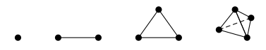
A simplicial complex \(K\) can be viewed as a purely combinatorial object, as described above, but it also gives rise to a topological space \(|K|\) (its geometric realization) as follows: first, the points of \(V\) should be in general position in euclidean space. Next, if \(\{v\}\) is in \(K\), then the vertex \(v\) is in \(|K|\). If \(\{v, w\}\) is in \(K\), then the line segment from \(v\) to \(w\) is in \(|K|\). If \(\{u, v, w\}\) is in \(K\), then the triangle with vertices \(u\), \(v\), and \(w\) is in \(|K|\). In general, \(|K|\) is the union of the convex hulls of simplices of \(K\). Frequently, one abuses notation and uses \(K\) to denote both the simplicial complex and the associated topological space.
For any simplicial complex \(K\) and any commutative ring \(R\) there is an associated chain complex, with differential of degree \(-1\). The \(n\)-th term is the free \(R\)-module with basis given by the \(n\)-simplices of \(K\). The differential is determined by its value on any simplex: on the \(n\)-simplex with vertices \((v_0, v_1, ..., v_n)\), the differential is the alternating sum with \(i\)-th summand \((-1)^i\) multiplied by the \((n-1)\)-simplex obtained by omitting vertex \(v_i\).
In the implementation here, the vertex set must be finite. To define a simplicial complex, specify its facets: the maximal subsets (with respect to inclusion) of the vertex set belonging to \(K\). Each facet can be specified as a list, a tuple, or a set.
Note
This class derives from
GenericCellComplex, and so
inherits its methods. Some of those methods are not listed here;
see the Generic Cell Complex
page instead.
EXAMPLES:
sage: SimplicialComplex([[1], [3, 7]])
Simplicial complex with vertex set (1, 3, 7) and facets {(1,), (3, 7)}
sage: SimplicialComplex()   # the empty simplicial complex
Simplicial complex with vertex set () and facets {()}
sage: X = SimplicialComplex([[0,1], [1,2], [2,3], [3,0]])
sage: X
Simplicial complex with vertex set (0, 1, 2, 3) and
 facets {(0, 1), (0, 3), (1, 2), (2, 3)}
>>> from sage.all import *
>>> SimplicialComplex([[Integer(1)], [Integer(3), Integer(7)]])
Simplicial complex with vertex set (1, 3, 7) and facets {(1,), (3, 7)}
>>> SimplicialComplex()   # the empty simplicial complex
Simplicial complex with vertex set () and facets {()}
>>> X = SimplicialComplex([[Integer(0),Integer(1)], [Integer(1),Integer(2)], [Integer(2),Integer(3)], [Integer(3),Integer(0)]])
>>> X
Simplicial complex with vertex set (0, 1, 2, 3) and
 facets {(0, 1), (0, 3), (1, 2), (2, 3)}
Sage can perform a number of operations on simplicial complexes, such as the join and the product, and it can also compute homology:
sage: S = SimplicialComplex([[0,1], [1,2], [0,2]]) # circle
sage: T = S.product(S)  # torus
sage: T
Simplicial complex with 9 vertices and 18 facets
sage: T.homology()   # this computes reduced homology                               # needs sage.modules
{0: 0, 1: Z x Z, 2: Z}
sage: T.euler_characteristic()
0
>>> from sage.all import *
>>> S = SimplicialComplex([[Integer(0),Integer(1)], [Integer(1),Integer(2)], [Integer(0),Integer(2)]]) # circle
>>> T = S.product(S)  # torus
>>> T
Simplicial complex with 9 vertices and 18 facets
>>> T.homology()   # this computes reduced homology                               # needs sage.modules
{0: 0, 1: Z x Z, 2: Z}
>>> T.euler_characteristic()
0
Sage knows about some basic combinatorial data associated to a simplicial complex:
sage: X = SimplicialComplex([[0,1], [1,2], [2,3], [0,3]])
sage: X.f_vector()
[1, 4, 4]
sage: X.face_poset()
Finite poset containing 8 elements
sage: x0, x1, x2, x3 = X.stanley_reisner_ring().gens()                              # needs sage.libs.singular
sage: x0*x2 == x1*x3 == 0                                                           # needs sage.libs.singular
True
sage: X.is_pure()
True
>>> from sage.all import *
>>> X = SimplicialComplex([[Integer(0),Integer(1)], [Integer(1),Integer(2)], [Integer(2),Integer(3)], [Integer(0),Integer(3)]])
>>> X.f_vector()
[1, 4, 4]
>>> X.face_poset()
Finite poset containing 8 elements
>>> x0, x1, x2, x3 = X.stanley_reisner_ring().gens()                              # needs sage.libs.singular
>>> x0*x2 == x1*x3 == Integer(0)                                                           # needs sage.libs.singular
True
>>> X.is_pure()
True
Mutability (see Issue #12587):
sage: S = SimplicialComplex([[1,4], [2,4]])
sage: S.add_face([1,3])
sage: S.remove_face([1,3]); S
Simplicial complex with vertex set (1, 2, 3, 4) and facets {(3,), (1, 4), (2, 4)}
sage: hash(S)
Traceback (most recent call last):
...
ValueError: this simplicial complex must be immutable; call set_immutable()
sage: S = SimplicialComplex([[1,4], [2,4]])
sage: S.set_immutable()
sage: S.add_face([1,3])
Traceback (most recent call last):
...
ValueError: this simplicial complex is not mutable
sage: S.remove_face([1,3])
Traceback (most recent call last):
...
ValueError: this simplicial complex is not mutable
sage: hash(S) == hash(S)
True

sage: S2 = SimplicialComplex([[1,4], [2,4]], is_mutable=False)
sage: hash(S2) == hash(S)
True
>>> from sage.all import *
>>> S = SimplicialComplex([[Integer(1),Integer(4)], [Integer(2),Integer(4)]])
>>> S.add_face([Integer(1),Integer(3)])
>>> S.remove_face([Integer(1),Integer(3)]); S
Simplicial complex with vertex set (1, 2, 3, 4) and facets {(3,), (1, 4), (2, 4)}
>>> hash(S)
Traceback (most recent call last):
...
ValueError: this simplicial complex must be immutable; call set_immutable()
>>> S = SimplicialComplex([[Integer(1),Integer(4)], [Integer(2),Integer(4)]])
>>> S.set_immutable()
>>> S.add_face([Integer(1),Integer(3)])
Traceback (most recent call last):
...
ValueError: this simplicial complex is not mutable
>>> S.remove_face([Integer(1),Integer(3)])
Traceback (most recent call last):
...
ValueError: this simplicial complex is not mutable
>>> hash(S) == hash(S)
True

>>> S2 = SimplicialComplex([[Integer(1),Integer(4)], [Integer(2),Integer(4)]], is_mutable=False)
>>> hash(S2) == hash(S)
True
We can also make mutable copies of an immutable simplicial complex (see Issue #14142):
sage: S = SimplicialComplex([[1,4], [2,4]])
sage: S.set_immutable()
sage: T = copy(S)
sage: T.is_mutable()
True
sage: S == T
True
>>> from sage.all import *
>>> S = SimplicialComplex([[Integer(1),Integer(4)], [Integer(2),Integer(4)]])
>>> S.set_immutable()
>>> T = copy(S)
>>> T.is_mutable()
True
>>> S == T
True
- class sage.topology.simplicial_complex.Simplex(X)[source]
Bases:
SageObjectDefine a simplex.
Topologically, a simplex is the convex hull of a collection of vertices in general position. Combinatorially, it is defined just by specifying a set of vertices. It is represented in Sage by the tuple of the vertices.
INPUT:
X– set of vertices (integer, list, or other iterable)
OUTPUT: simplex with those vertices
Xmay be a nonnegative integer \(n\), in which case the simplicial complex will have \(n+1\) vertices \((0, 1, ..., n)\), or it may be anything which may be converted to a tuple, in which case the vertices will be that tuple. In the second case, each vertex must be hashable, so it should be a number, a string, or a tuple, for instance, but not a list.Warning
The vertices should be distinct, and no error checking is done to make sure this is the case.
EXAMPLES:
sage: Simplex(4)
(0, 1, 2, 3, 4)
sage: Simplex([3, 4, 1])
(3, 4, 1)
sage: X = Simplex((3, 'a', 'vertex')); X
(3, 'a', 'vertex')
sage: X == loads(dumps(X))
True
>>> from sage.all import *
>>> Simplex(Integer(4))
(0, 1, 2, 3, 4)
>>> Simplex([Integer(3), Integer(4), Integer(1)])
(3, 4, 1)
>>> X = Simplex((Integer(3), 'a', 'vertex')); X
(3, 'a', 'vertex')
>>> X == loads(dumps(X))
True
Vertices may be tuples but not lists:
sage: Simplex([(1,2), (3,4)])
((1, 2), (3, 4))
sage: Simplex([[1,2], [3,4]])
Traceback (most recent call last):
...
TypeError: ...unhashable type: 'list'...
>>> from sage.all import *
>>> Simplex([(Integer(1),Integer(2)), (Integer(3),Integer(4))])
((1, 2), (3, 4))
>>> Simplex([[Integer(1),Integer(2)], [Integer(3),Integer(4)]])
Traceback (most recent call last):
...
TypeError: ...unhashable type: 'list'...
- alexander_whitney(dim)[source]
Subdivide this simplex into a pair of simplices.
If this simplex has vertices \(v_0\), \(v_1\), …, \(v_n\), then subdivide it into simplices \((v_0, v_1, ..., v_{dim})\) and \((v_{dim}, v_{dim + 1}, ..., v_n)\).
INPUT:
dim– integer between 0 and one more than the dimension of this simplex
OUTPUT:
a list containing just the triple
(1, left, right), whereleftandrightare the two simplices described above.
This method allows one to construct a coproduct from the \(p+q\)-chains to the tensor product of the \(p\)-chains and the \(q\)-chains. The number 1 (a Sage integer) is the coefficient of
left tensor rightin this coproduct. (The corresponding formula is more complicated for the cubes that make up a cubical complex, and the output format is intended to be consistent for both cubes and simplices.)Calling this method
alexander_whitneyis an abuse of notation, since the actual Alexander-Whitney map goes from \(C(X \times Y) \to C(X) \otimes C(Y)\), where \(C(-)\) denotes the chain complex of singular chains, but this subdivision of simplices is at the heart of it.EXAMPLES:
sage: s = Simplex((0,1,3,4))
sage: s.alexander_whitney(0)
[(1, (0,), (0, 1, 3, 4))]
sage: s.alexander_whitney(2)
[(1, (0, 1, 3), (3, 4))]
>>> from sage.all import *
>>> s = Simplex((Integer(0),Integer(1),Integer(3),Integer(4)))
>>> s.alexander_whitney(Integer(0))
[(1, (0,), (0, 1, 3, 4))]
>>> s.alexander_whitney(Integer(2))
[(1, (0, 1, 3), (3, 4))]
- dimension()[source]
The dimension of this simplex.
The dimension of a simplex is the number of vertices minus 1.
EXAMPLES:
sage: Simplex(5).dimension() == 5
True
sage: Simplex(5).face(1).dimension()
4
>>> from sage.all import *
>>> Simplex(Integer(5)).dimension() == Integer(5)
True
>>> Simplex(Integer(5)).face(Integer(1)).dimension()
4
- face(n)[source]
The \(n\)-th face of this simplex.
INPUT:
n– integer between 0 and the dimension of this simplex
OUTPUT: the simplex obtained by removing the \(n\)-th vertex from this simplex
EXAMPLES:
sage: S = Simplex(4)
sage: S.face(0)
(1, 2, 3, 4)
sage: S.face(3)
(0, 1, 2, 4)
>>> from sage.all import *
>>> S = Simplex(Integer(4))
>>> S.face(Integer(0))
(1, 2, 3, 4)
>>> S.face(Integer(3))
(0, 1, 2, 4)
- faces()[source]
The list of faces (of codimension 1) of this simplex.
EXAMPLES:
sage: S = Simplex(4)
sage: S.faces()
[(1, 2, 3, 4), (0, 2, 3, 4), (0, 1, 3, 4), (0, 1, 2, 4), (0, 1, 2, 3)]
sage: len(Simplex(10).faces())
11
>>> from sage.all import *
>>> S = Simplex(Integer(4))
>>> S.faces()
[(1, 2, 3, 4), (0, 2, 3, 4), (0, 1, 3, 4), (0, 1, 2, 4), (0, 1, 2, 3)]
>>> len(Simplex(Integer(10)).faces())
11
- is_empty()[source]
Return
Trueiff this simplex is the empty simplex.EXAMPLES:
sage: [Simplex(n).is_empty() for n in range(-1,4)]
[True, False, False, False, False]
>>> from sage.all import *
>>> [Simplex(n).is_empty() for n in range(-Integer(1),Integer(4))]
[True, False, False, False, False]
- is_face(other)[source]
Return
Trueiff this simplex is a face of other.EXAMPLES:
sage: Simplex(3).is_face(Simplex(5))
True
sage: Simplex(5).is_face(Simplex(2))
False
sage: Simplex(['a', 'b', 'c']).is_face(Simplex(8))
False
>>> from sage.all import *
>>> Simplex(Integer(3)).is_face(Simplex(Integer(5)))
True
>>> Simplex(Integer(5)).is_face(Simplex(Integer(2)))
False
>>> Simplex(['a', 'b', 'c']).is_face(Simplex(Integer(8)))
False
- join(right, rename_vertices=True)[source]
The join of this simplex with another one.
The join of two simplices \([v_0, ..., v_k]\) and \([w_0, ..., w_n]\) is the simplex \([v_0, ..., v_k, w_0, ..., w_n]\).
INPUT:
right– the other simplex (the right-hand factor)rename_vertices– boolean (default:True); if this isTrue, the vertices in the join will be renamed by this formula: vertex “v” in the left-hand factor –> vertex “Lv” in the join, vertex “w” in the right-hand factor –> vertex “Rw” in the join. If this isFalse, this tries to construct the join without renaming the vertices; this may cause problems if the two factors have any vertices with names in common.
EXAMPLES:
sage: Simplex(2).join(Simplex(3))
('L0', 'L1', 'L2', 'R0', 'R1', 'R2', 'R3')
sage: Simplex(['a', 'b']).join(Simplex(['x', 'y', 'z']))
('La', 'Lb', 'Rx', 'Ry', 'Rz')
sage: Simplex(['a', 'b']).join(Simplex(['x', 'y', 'z']), rename_vertices=False)
('a', 'b', 'x', 'y', 'z')
>>> from sage.all import *
>>> Simplex(Integer(2)).join(Simplex(Integer(3)))
('L0', 'L1', 'L2', 'R0', 'R1', 'R2', 'R3')
>>> Simplex(['a', 'b']).join(Simplex(['x', 'y', 'z']))
('La', 'Lb', 'Rx', 'Ry', 'Rz')
>>> Simplex(['a', 'b']).join(Simplex(['x', 'y', 'z']), rename_vertices=False)
('a', 'b', 'x', 'y', 'z')
- product(other, rename_vertices=True)[source]
The product of this simplex with another one, as a list of simplices.
INPUT:
other– the other simplexrename_vertices– boolean (default:True); if this isFalse, then the vertices in the product are the set of ordered pairs \((v,w)\) where \(v\) is a vertex in the left-hand factor (self) and \(w\) is a vertex in the right-hand factor (other). If this isTrue, then the vertices are renamed as “LvRw” (e.g., the vertex (1,2) would become “L1R2”). This is useful if you want to define the Stanley-Reisner ring of the complex: vertex names like (0,1) are not suitable for that, while vertex names like “L0R1” are.
ALGORITHM: see Hatcher, p. 277-278 [Hat2002] (who in turn refers to Eilenberg-Steenrod, p. 68): given
S = Simplex(m)andT = Simplex(n), then \(S \times T\) can be triangulated as follows: for each path \(f\) from \((0,0)\) to \((m,n)\) along the integer grid in the plane, going up or right at each lattice point, associate an \((m+n)\)-simplex with vertices \(v_0\), \(v_1\), …, where \(v_k\) is the \(k\)-th vertex in the path \(f\).Note that there are \(m+n\) choose \(n\) such paths. Note also that each vertex in the product is a pair of vertices \((v,w)\) where \(v\) is a vertex in the left-hand factor and \(w\) is a vertex in the right-hand factor.
Note
This produces a list of simplices – not a
Simplex, not aSimplicialComplex.EXAMPLES:
sage: len(Simplex(2).product(Simplex(2)))
6
sage: Simplex(1).product(Simplex(1))
[('L0R0', 'L0R1', 'L1R1'), ('L0R0', 'L1R0', 'L1R1')]
sage: Simplex(1).product(Simplex(1), rename_vertices=False)
[((0, 0), (0, 1), (1, 1)), ((0, 0), (1, 0), (1, 1))]
>>> from sage.all import *
>>> len(Simplex(Integer(2)).product(Simplex(Integer(2))))
6
>>> Simplex(Integer(1)).product(Simplex(Integer(1)))
[('L0R0', 'L0R1', 'L1R1'), ('L0R0', 'L1R0', 'L1R1')]
>>> Simplex(Integer(1)).product(Simplex(Integer(1)), rename_vertices=False)
[((0, 0), (0, 1), (1, 1)), ((0, 0), (1, 0), (1, 1))]
- set()[source]
The frozenset attached to this simplex.
EXAMPLES:
sage: Simplex(3).set()
frozenset({0, 1, 2, 3})
>>> from sage.all import *
>>> Simplex(Integer(3)).set()
frozenset({0, 1, 2, 3})
- tuple()[source]
The tuple attached to this simplex.
EXAMPLES:
sage: Simplex(3).tuple()
(0, 1, 2, 3)
>>> from sage.all import *
>>> Simplex(Integer(3)).tuple()
(0, 1, 2, 3)
Although simplices are printed as if they were tuples, they are not the same type:
sage: type(Simplex(3).tuple())
<... 'tuple'>
sage: type(Simplex(3))
<class 'sage.topology.simplicial_complex.Simplex'>
>>> from sage.all import *
>>> type(Simplex(Integer(3)).tuple())
<... 'tuple'>
>>> type(Simplex(Integer(3)))
<class 'sage.topology.simplicial_complex.Simplex'>
- class sage.topology.simplicial_complex.SimplicialComplex(maximal_faces=None, from_characteristic_function=None, maximality_check=True, sort_facets=None, name_check=False, is_mutable=True, is_immutable=False, category=None)[source]
Bases:
Parent,GenericCellComplexDefine a simplicial complex.
INPUT:
maximal_faces– set of maximal facesfrom_characteristic_function– see belowmaximality_check– boolean (default:True); see belowsort_facets– dictionary; see belowname_check– boolean (default:False); see belowis_mutable– boolean (default:True); set toFalseto make this immutablecategory– the category of the simplicial complex (default: finite simplicial complexes)
OUTPUT: a simplicial complex
maximal_facesshould be a list or tuple or set (indeed, anything which may be converted to a set) whose elements are lists (or tuples, etc.) of vertices. Maximal faces are also known as ‘facets’.maximal_facescan also be a list containing a single nonnegative integer \(n\), in which case this constructs the simplicial complex with a single \(n\)-simplex as the only facet.Alternatively, the maximal faces can be defined from a monotone boolean function on the subsets of a set \(X\). While defining
maximal_faces=None, you can thus setfrom_characteristic_function=(f,X)whereXis the set of points andfa boolean monotone hereditary function that accepts a list of elements fromXas input (seesubsets_with_hereditary_property()for more information).If
maximality_checkisTrue, check that each maximal face is, in fact, maximal. In this case, when producing the internal representation of the simplicial complex, omit those that are not. It is highly recommended that this beTrue; various methods for this class may fail if faces which are claimed to be maximal are in fact not.sort_facets: if not set toNone, the default, this should be a dictionary, used for sorting the vertices in each facet. The keys must be the vertices for the simplicial complex, and the values should be distinct sortable objects, for example integers. This should not need to be specified except in very special circumstances; currently the only use in the Sage library is when defining the product of a simplicial complex with itself: in this case, the vertices in the product must be sorted compatibly with the vertices in each factor so that the diagonal map is properly defined.If
name_checkisTrue, check the names of the vertices to see if they can be easily converted to generators of a polynomial ring – use this if you plan to use the Stanley-Reisner ring for the simplicial complex.EXAMPLES:
sage: SimplicialComplex([[1,2], [1,4]])
Simplicial complex with vertex set (1, 2, 4) and facets {(1, 2), (1, 4)}
sage: SimplicialComplex([[0,2], [0,3], [0]])
Simplicial complex with vertex set (0, 2, 3) and facets {(0, 2), (0, 3)}
sage: SimplicialComplex([[0,2], [0,3], [0]], maximality_check=False)
Simplicial complex with vertex set (0, 2, 3) and facets {(0,), (0, 2), (0, 3)}
>>> from sage.all import *
>>> SimplicialComplex([[Integer(1),Integer(2)], [Integer(1),Integer(4)]])
Simplicial complex with vertex set (1, 2, 4) and facets {(1, 2), (1, 4)}
>>> SimplicialComplex([[Integer(0),Integer(2)], [Integer(0),Integer(3)], [Integer(0)]])
Simplicial complex with vertex set (0, 2, 3) and facets {(0, 2), (0, 3)}
>>> SimplicialComplex([[Integer(0),Integer(2)], [Integer(0),Integer(3)], [Integer(0)]], maximality_check=False)
Simplicial complex with vertex set (0, 2, 3) and facets {(0,), (0, 2), (0, 3)}
Finally, if the first argument is a simplicial complex, return that complex. If it is an object with a built-in conversion to simplicial complexes (via a
_simplicial_method), then the resulting simplicial complex is returned:sage: S = SimplicialComplex([[0,2], [0,3], [0,6]]) sage: SimplicialComplex(S) == S True sage: Tc = cubical_complexes.Torus(); Tc Cubical complex with 16 vertices and 64 cubes sage: Ts = SimplicialComplex(Tc); Ts Simplicial complex with 16 vertices and 32 facets sage: Ts.homology() # needs sage.modules {0: 0, 1: Z x Z, 2: Z}
>>> from sage.all import *
>>> S = SimplicialComplex([[Integer(0),Integer(2)], [Integer(0),Integer(3)], [Integer(0),Integer(6)]])
>>> SimplicialComplex(S) == S
True
>>> Tc = cubical_complexes.Torus(); Tc
Cubical complex with 16 vertices and 64 cubes
>>> Ts = SimplicialComplex(Tc); Ts
Simplicial complex with 16 vertices and 32 facets
>>> Ts.homology()                                                             # needs sage.modules
{0: 0, 1: Z x Z, 2: Z}
In the situation where the first argument is a simplicial complex or another object with a built-in conversion, most of the other arguments are ignored. The only exception is
is_mutable:sage: S.is_mutable() True sage: SimplicialComplex(S, is_mutable=False).is_mutable() False
>>> from sage.all import *
>>> S.is_mutable()
True
>>> SimplicialComplex(S, is_mutable=False).is_mutable()
False
From a characteristic monotone boolean function, e.g. the simplicial complex of all subsets \(S\subseteq \{0,1,2,3,4\}\) such that \(sum(S)\leq 4\):
sage: SimplicialComplex(from_characteristic_function=(lambda x:sum(x)<=4, range(5)))
Simplicial complex with vertex set (0, 1, 2, 3, 4) and facets {(0, 4), (0, 1, 2), (0, 1, 3)}
>>> from sage.all import *
>>> SimplicialComplex(from_characteristic_function=(lambda x:sum(x)<=Integer(4), range(Integer(5))))
Simplicial complex with vertex set (0, 1, 2, 3, 4) and facets {(0, 4), (0, 1, 2), (0, 1, 3)}
or e.g. the simplicial complex of all 168 hyperovals of the projective plane of order 4:
sage: l = designs.ProjectiveGeometryDesign(2, 1, GF(4,name='a'))                # needs sage.rings.finite_rings
sage: f = lambda S: not any(len(set(S).intersection(x))>2 for x in l)
sage: SimplicialComplex(from_characteristic_function=(f, l.ground_set()))       # needs sage.rings.finite_rings, long time
Simplicial complex with 21 vertices and 168 facets
>>> from sage.all import *
>>> l = designs.ProjectiveGeometryDesign(Integer(2), Integer(1), GF(Integer(4),name='a'))                # needs sage.rings.finite_rings
>>> f = lambda S: not any(len(set(S).intersection(x))>Integer(2) for x in l)
>>> SimplicialComplex(from_characteristic_function=(f, l.ground_set()))       # needs sage.rings.finite_rings, long time
Simplicial complex with 21 vertices and 168 facets
Warning
Simplicial complexes are not proper parents as they do not possess element classes. In particular, parents are assumed to be hashable (and hence immutable) by the coercion framework. However this is close enough to being a parent with elements being the faces of
selfthat we currently allow this abuse.- F_triangle(S)[source]
Return the F-triangle of
selfwith respect to one maximal simplexS.This is the bivariate generating polynomial of all faces, according to the number of elements in
Sand outsideS.OUTPUT: an
F_triangleSee also
Not to be confused with
f_triangle().EXAMPLES:
sage: cs = simplicial_complexes.Torus()
sage: cs.F_triangle(cs.facets()[0])                                         # needs sage.combinat
F: x^3 + 9*x^2*y + 3*x*y^2 + y^3 + 6*x^2 + 12*x*y
+ 3*y^2 + 4*x + 3*y + 1
>>> from sage.all import *
>>> cs = simplicial_complexes.Torus()
>>> cs.F_triangle(cs.facets()[Integer(0)])                                         # needs sage.combinat
F: x^3 + 9*x^2*y + 3*x*y^2 + y^3 + 6*x^2 + 12*x*y
+ 3*y^2 + 4*x + 3*y + 1
- add_face(face)[source]
Add a face to this simplicial complex.
INPUT:
face– a subset of the vertex set
This changes the simplicial complex, adding a new face and all of its subfaces.
EXAMPLES:
sage: X = SimplicialComplex([[0,1], [0,2]])
sage: X.add_face([0,1,2,]); X
Simplicial complex with vertex set (0, 1, 2) and facets {(0, 1, 2)}
sage: Y = SimplicialComplex(); Y
Simplicial complex with vertex set () and facets {()}
sage: Y.add_face([0,1])
sage: Y.add_face([1,2,3])
sage: Y
Simplicial complex with vertex set (0, 1, 2, 3) and facets {(0, 1), (1, 2, 3)}
>>> from sage.all import *
>>> X = SimplicialComplex([[Integer(0),Integer(1)], [Integer(0),Integer(2)]])
>>> X.add_face([Integer(0),Integer(1),Integer(2),]); X
Simplicial complex with vertex set (0, 1, 2) and facets {(0, 1, 2)}
>>> Y = SimplicialComplex(); Y
Simplicial complex with vertex set () and facets {()}
>>> Y.add_face([Integer(0),Integer(1)])
>>> Y.add_face([Integer(1),Integer(2),Integer(3)])
>>> Y
Simplicial complex with vertex set (0, 1, 2, 3) and facets {(0, 1), (1, 2, 3)}
If you add a face which is already present, there is no effect:
sage: Y.add_face([1,3]); Y
Simplicial complex with vertex set (0, 1, 2, 3) and facets {(0, 1), (1, 2, 3)}
>>> from sage.all import *
>>> Y.add_face([Integer(1),Integer(3)]); Y
Simplicial complex with vertex set (0, 1, 2, 3) and facets {(0, 1), (1, 2, 3)}
- alexander_dual(is_mutable=True)[source]
The Alexander dual of this simplicial complex: according to the Macaulay2 documentation, this is the simplicial complex whose faces are the complements of its nonfaces.
Thus find the minimal nonfaces and take their complements to find the facets in the Alexander dual.
INPUT:
is_mutable– boolean (default:True); determine whether the output is mutable
EXAMPLES:
sage: Y = SimplicialComplex([[i] for i in range(5)]); Y
Simplicial complex with vertex set (0, 1, 2, 3, 4) and
 facets {(0,), (1,), (2,), (3,), (4,)}
sage: Y.alexander_dual()
Simplicial complex with vertex set (0, 1, 2, 3, 4) and 10 facets
sage: X = SimplicialComplex([[0,1], [1,2], [2,3], [3,0]])
sage: X.alexander_dual()
Simplicial complex with vertex set (0, 1, 2, 3) and facets {(0, 2), (1, 3)}
>>> from sage.all import *
>>> Y = SimplicialComplex([[i] for i in range(Integer(5))]); Y
Simplicial complex with vertex set (0, 1, 2, 3, 4) and
 facets {(0,), (1,), (2,), (3,), (4,)}
>>> Y.alexander_dual()
Simplicial complex with vertex set (0, 1, 2, 3, 4) and 10 facets
>>> X = SimplicialComplex([[Integer(0),Integer(1)], [Integer(1),Integer(2)], [Integer(2),Integer(3)], [Integer(3),Integer(0)]])
>>> X.alexander_dual()
Simplicial complex with vertex set (0, 1, 2, 3) and facets {(0, 2), (1, 3)}
- alexander_whitney(simplex, dim_left)[source]
Subdivide this simplex into a pair of simplices.
If this simplex has vertices \(v_0\), \(v_1\), …, \(v_n\), then subdivide it into simplices \((v_0, v_1, ..., v_{dim})\) and \((v_{dim}, v_{dim + 1}, ..., v_n)\).
See
Simplex.alexander_whitney()for more details. This method just calls that one.INPUT:
simplex– a simplex in this complexdim– integer between 0 and one more than the dimension of this simplex
OUTPUT: list containing just the triple
(1, left,
right)
, whereleftandrightare the two simplices described above.EXAMPLES:
sage: s = Simplex((0,1,3,4))
sage: X = SimplicialComplex([s])
sage: X.alexander_whitney(s, 0)
[(1, (0,), (0, 1, 3, 4))]
sage: X.alexander_whitney(s, 2)
[(1, (0, 1, 3), (3, 4))]
>>> from sage.all import *
>>> s = Simplex((Integer(0),Integer(1),Integer(3),Integer(4)))
>>> X = SimplicialComplex([s])
>>> X.alexander_whitney(s, Integer(0))
[(1, (0,), (0, 1, 3, 4))]
>>> X.alexander_whitney(s, Integer(2))
[(1, (0, 1, 3), (3, 4))]
- algebraic_topological_model(base_ring=None)[source]
Algebraic topological model for this simplicial complex with coefficients in
base_ring.The term “algebraic topological model” is defined by Pilarczyk and Réal [PR2015].
INPUT:
base_ring– coefficient ring (default:QQ); must be a field
Denote by \(C\) the chain complex associated to this simplicial complex. The algebraic topological model is a chain complex \(M\) with zero differential, with the same homology as \(C\), along with chain maps \(\pi: C \to M\) and \(\iota: M \to C\) satisfying \(\iota \pi = 1_M\) and \(\pi \iota\) chain homotopic to \(1_C\). The chain homotopy \(\phi\) must satisfy
\(\phi \phi = 0\),
\(\pi \phi = 0\),
\(\phi \iota = 0\).
Such a chain homotopy is called a chain contraction.
OUTPUT: a pair consisting of
chain contraction
phiassociated to \(C\), \(M\), \(\pi\), and \(\iota\)the chain complex \(M\)
Note that from the chain contraction
phi, one can recover the chain maps \(\pi\) and \(\iota\) viaphi.pi()andphi.iota(). Then one can recover \(C\) and \(M\) from, for example,phi.pi().domain()andphi.pi().codomain(), respectively.EXAMPLES:
sage: # needs sage.modules
sage: RP2 = simplicial_complexes.RealProjectivePlane()
sage: phi, M = RP2.algebraic_topological_model(GF(2))
sage: M.homology()
{0: Vector space of dimension 1 over Finite Field of size 2,
 1: Vector space of dimension 1 over Finite Field of size 2,
 2: Vector space of dimension 1 over Finite Field of size 2}
sage: T = simplicial_complexes.Torus()
sage: phi, M = T.algebraic_topological_model(QQ)
sage: M.homology()
{0: Vector space of dimension 1 over Rational Field,
 1: Vector space of dimension 2 over Rational Field,
 2: Vector space of dimension 1 over Rational Field}
>>> from sage.all import *
>>> # needs sage.modules
>>> RP2 = simplicial_complexes.RealProjectivePlane()
>>> phi, M = RP2.algebraic_topological_model(GF(Integer(2)))
>>> M.homology()
{0: Vector space of dimension 1 over Finite Field of size 2,
 1: Vector space of dimension 1 over Finite Field of size 2,
 2: Vector space of dimension 1 over Finite Field of size 2}
>>> T = simplicial_complexes.Torus()
>>> phi, M = T.algebraic_topological_model(QQ)
>>> M.homology()
{0: Vector space of dimension 1 over Rational Field,
 1: Vector space of dimension 2 over Rational Field,
 2: Vector space of dimension 1 over Rational Field}
- automorphism_group()[source]
Return the automorphism group of the simplicial complex.
This is done by creating a bipartite graph, whose vertices are vertices and facets of the simplicial complex, and computing its automorphism group.
Warning
Since Issue #14319 the domain of the automorphism group is equal to the graph’s vertex set, and the
translationargument has become useless.EXAMPLES:
sage: S = simplicial_complexes.Simplex(3)
sage: S.automorphism_group().is_isomorphic(SymmetricGroup(4))               # needs sage.groups
True

sage: P = simplicial_complexes.RealProjectivePlane()
sage: P.automorphism_group().is_isomorphic(AlternatingGroup(5))             # needs sage.groups
True

sage: Z = SimplicialComplex([['1','2'],['2','3','a']])
sage: Z.automorphism_group().is_isomorphic(CyclicPermutationGroup(2))       # needs sage.groups
True
sage: group = Z.automorphism_group()                                        # needs sage.groups
sage: sorted(group.domain())                                                # needs sage.groups
['1', '2', '3', 'a']
>>> from sage.all import *
>>> S = simplicial_complexes.Simplex(Integer(3))
>>> S.automorphism_group().is_isomorphic(SymmetricGroup(Integer(4)))               # needs sage.groups
True

>>> P = simplicial_complexes.RealProjectivePlane()
>>> P.automorphism_group().is_isomorphic(AlternatingGroup(Integer(5)))             # needs sage.groups
True

>>> Z = SimplicialComplex([['1','2'],['2','3','a']])
>>> Z.automorphism_group().is_isomorphic(CyclicPermutationGroup(Integer(2)))       # needs sage.groups
True
>>> group = Z.automorphism_group()                                        # needs sage.groups
>>> sorted(group.domain())                                                # needs sage.groups
['1', '2', '3', 'a']
Check that Issue #17032 is fixed:
sage: s = SimplicialComplex([[(0,1),(2,3)]])
sage: s.automorphism_group().cardinality()                                  # needs sage.groups
2
>>> from sage.all import *
>>> s = SimplicialComplex([[(Integer(0),Integer(1)),(Integer(2),Integer(3))]])
>>> s.automorphism_group().cardinality()                                  # needs sage.groups
2
- barycentric_subdivision()[source]
The barycentric subdivision of this simplicial complex.
See Wikipedia article Barycentric_subdivision for a definition.
EXAMPLES:
sage: triangle = SimplicialComplex([[0,1], [1,2], [0, 2]])
sage: hexagon = triangle.barycentric_subdivision(); hexagon
Simplicial complex with 6 vertices and 6 facets
sage: hexagon.homology(1) == triangle.homology(1)                           # needs sage.modules
True
>>> from sage.all import *
>>> triangle = SimplicialComplex([[Integer(0),Integer(1)], [Integer(1),Integer(2)], [Integer(0), Integer(2)]])
>>> hexagon = triangle.barycentric_subdivision(); hexagon
Simplicial complex with 6 vertices and 6 facets
>>> hexagon.homology(Integer(1)) == triangle.homology(Integer(1))                           # needs sage.modules
True
Barycentric subdivisions can get quite large, since each \(n\)-dimensional facet in the original complex produces \((n+1)!\) facets in the subdivision:
sage: S4 = simplicial_complexes.Sphere(4); S4
Minimal triangulation of the 4-sphere
sage: S4.barycentric_subdivision()
Simplicial complex with 62 vertices and 720 facets
>>> from sage.all import *
>>> S4 = simplicial_complexes.Sphere(Integer(4)); S4
Minimal triangulation of the 4-sphere
>>> S4.barycentric_subdivision()
Simplicial complex with 62 vertices and 720 facets
- bigraded_betti_number(a, b, base_ring=Integer Ring, verbose=False)[source]
Return the bigraded Betti number indexed in the form \((-a, 2b)\).
Bigraded Betti number with indices \((-a, 2b)\) is defined as a sum of ranks of \((b-a-1)\)-th (co)homologies of full subcomplexes with exactly \(b\) vertices.
INPUT:
base_ring– (default:ZZ) the base ring used when computing homologyverbose– boolean (default:False); ifTrue, print messages during the computation, which indicate in which subcomplexes non-trivial homologies appear
Note
If
verboseisTrue, then caching is avoided.EXAMPLES:
sage: # needs sage.modules
sage: X = SimplicialComplex([[0,1],[1,2],[2,0],[1,3]])
sage: X.bigraded_betti_number(-1, 4, base_ring=QQ)
2
sage: X.bigraded_betti_number(-1, 8)
0
sage: X.bigraded_betti_number(-2, 5)
0
sage: X.bigraded_betti_number(0, 0)
1
sage: sorted(X.bigraded_betti_numbers().items(), reverse=True)
[((0, 0), 1), ((-1, 6), 1), ((-1, 4), 2), ((-2, 8), 1), ((-2, 6), 1)]
sage: X.bigraded_betti_number(-1, 4, base_ring=QQ)
2
sage: X.bigraded_betti_number(-1, 8)
0
sage: Y = SimplicialComplex([[1,2,3],[1,2,4],[3,5],[4,5]])
sage: Y.bigraded_betti_number(-1, 4, verbose=True)
Non-trivial homology Z in dimension 0 of the full subcomplex
generated by a set of vertices (1, 5)
Non-trivial homology Z in dimension 0 of the full subcomplex
generated by a set of vertices (2, 5)
Non-trivial homology Z in dimension 0 of the full subcomplex
generated by a set of vertices (3, 4)
3
>>> from sage.all import *
>>> # needs sage.modules
>>> X = SimplicialComplex([[Integer(0),Integer(1)],[Integer(1),Integer(2)],[Integer(2),Integer(0)],[Integer(1),Integer(3)]])
>>> X.bigraded_betti_number(-Integer(1), Integer(4), base_ring=QQ)
2
>>> X.bigraded_betti_number(-Integer(1), Integer(8))
0
>>> X.bigraded_betti_number(-Integer(2), Integer(5))
0
>>> X.bigraded_betti_number(Integer(0), Integer(0))
1
>>> sorted(X.bigraded_betti_numbers().items(), reverse=True)
[((0, 0), 1), ((-1, 6), 1), ((-1, 4), 2), ((-2, 8), 1), ((-2, 6), 1)]
>>> X.bigraded_betti_number(-Integer(1), Integer(4), base_ring=QQ)
2
>>> X.bigraded_betti_number(-Integer(1), Integer(8))
0
>>> Y = SimplicialComplex([[Integer(1),Integer(2),Integer(3)],[Integer(1),Integer(2),Integer(4)],[Integer(3),Integer(5)],[Integer(4),Integer(5)]])
>>> Y.bigraded_betti_number(-Integer(1), Integer(4), verbose=True)
Non-trivial homology Z in dimension 0 of the full subcomplex
generated by a set of vertices (1, 5)
Non-trivial homology Z in dimension 0 of the full subcomplex
generated by a set of vertices (2, 5)
Non-trivial homology Z in dimension 0 of the full subcomplex
generated by a set of vertices (3, 4)
3
- bigraded_betti_numbers(base_ring=Integer Ring, verbose=False)[source]
Return a dictionary of the bigraded Betti numbers of
self, with keys \((-a, 2b)\).INPUT:
base_ring– (default:ZZ) the base ring used when computing homologyverbose– boolean (default:False); ifTrue, print messages during the computation, which indicate in which subcomplexes non-trivial homologies appear
Note
If
verboseisTrue, then caching is avoided.See also
See
bigraded_betti_number()for more information.EXAMPLES:
sage: X = SimplicialComplex([[0,1],[1,2],[1,3],[2,3]])
sage: Y = SimplicialComplex([[1,2,3],[1,2,4],[3,5],[4,5]])
sage: sorted(X.bigraded_betti_numbers(base_ring=QQ).items(), reverse=True)
[((0, 0), 1), ((-1, 6), 1), ((-1, 4), 2), ((-2, 8), 1), ((-2, 6), 1)]
sage: sorted(Y.bigraded_betti_numbers(verbose=True).items(), reverse=True)
(-1, 4): Non-trivial homology Z in dimension 0 of the full
subcomplex generated by a set of vertices (1, 5)
(-1, 4): Non-trivial homology Z in dimension 0 of the full
subcomplex generated by a set of vertices (2, 5)
(-1, 4): Non-trivial homology Z in dimension 0 of the full
subcomplex generated by a set of vertices (3, 4)
(-2, 6): Non-trivial homology Z in dimension 0 of the full
subcomplex generated by a set of vertices (1, 2, 5)
(-2, 8): Non-trivial homology Z in dimension 1 of the full
subcomplex generated by a set of vertices (1, 3, 4, 5)
(-2, 8): Non-trivial homology Z in dimension 1 of the full
subcomplex generated by a set of vertices (2, 3, 4, 5)
(-3, 10): Non-trivial homology Z in dimension 1 of the full
subcomplex generated by a set of vertices (1, 2, 3, 4, 5)
[((0, 0), 1), ((-1, 4), 3), ((-2, 8), 2), ((-2, 6), 1), ((-3, 10), 1)]
>>> from sage.all import *
>>> X = SimplicialComplex([[Integer(0),Integer(1)],[Integer(1),Integer(2)],[Integer(1),Integer(3)],[Integer(2),Integer(3)]])
>>> Y = SimplicialComplex([[Integer(1),Integer(2),Integer(3)],[Integer(1),Integer(2),Integer(4)],[Integer(3),Integer(5)],[Integer(4),Integer(5)]])
>>> sorted(X.bigraded_betti_numbers(base_ring=QQ).items(), reverse=True)
[((0, 0), 1), ((-1, 6), 1), ((-1, 4), 2), ((-2, 8), 1), ((-2, 6), 1)]
>>> sorted(Y.bigraded_betti_numbers(verbose=True).items(), reverse=True)
(-1, 4): Non-trivial homology Z in dimension 0 of the full
subcomplex generated by a set of vertices (1, 5)
(-1, 4): Non-trivial homology Z in dimension 0 of the full
subcomplex generated by a set of vertices (2, 5)
(-1, 4): Non-trivial homology Z in dimension 0 of the full
subcomplex generated by a set of vertices (3, 4)
(-2, 6): Non-trivial homology Z in dimension 0 of the full
subcomplex generated by a set of vertices (1, 2, 5)
(-2, 8): Non-trivial homology Z in dimension 1 of the full
subcomplex generated by a set of vertices (1, 3, 4, 5)
(-2, 8): Non-trivial homology Z in dimension 1 of the full
subcomplex generated by a set of vertices (2, 3, 4, 5)
(-3, 10): Non-trivial homology Z in dimension 1 of the full
subcomplex generated by a set of vertices (1, 2, 3, 4, 5)
[((0, 0), 1), ((-1, 4), 3), ((-2, 8), 2), ((-2, 6), 1), ((-3, 10), 1)]
If we wish to view them in a form of a table, it is simple enough to create a function as such:
sage: def print_table(bbns):
....:     max_a = max(-p[0] for p in bbns)
....:     max_b = max(p[1] for p in bbns)
....:     bbn_table = [[bbns.get((-a,b), 0) for a in range(max_a+1)]
....:                                       for b in range(max_b+1)]
....:     width = len(str(max(bbns.values()))) + 1
....:     print(' '*width, end=' ')
....:     for i in range(max_a+1):
....:         print(f'{-i:{width}}', end=' ')
....:     print()
....:     for j in range(len(bbn_table)):
....:         print(f'{j:{width}}', end=' ')
....:         for r in bbn_table[j]:
....:             print(f'{r:{width}}', end=' ')
....:         print()
sage: print_table(X.bigraded_betti_numbers())
    0 -1 -2
 0  1  0  0
 1  0  0  0
 2  0  0  0
 3  0  0  0
 4  0  2  0
 5  0  0  0
 6  0  1  1
 7  0  0  0
 8  0  0  1
>>> from sage.all import *
>>> def print_table(bbns):
...     max_a = max(-p[Integer(0)] for p in bbns)
...     max_b = max(p[Integer(1)] for p in bbns)
...     bbn_table = [[bbns.get((-a,b), Integer(0)) for a in range(max_a+Integer(1))]
...                                       for b in range(max_b+Integer(1))]
...     width = len(str(max(bbns.values()))) + Integer(1)
...     print(' '*width, end=' ')
...     for i in range(max_a+Integer(1)):
...         print(f'{-i:{width}}', end=' ')
...     print()
...     for j in range(len(bbn_table)):
...         print(f'{j:{width}}', end=' ')
...         for r in bbn_table[j]:
...             print(f'{r:{width}}', end=' ')
...         print()
>>> print_table(X.bigraded_betti_numbers())
    0 -1 -2
 0  1  0  0
 1  0  0  0
 2  0  0  0
 3  0  0  0
 4  0  2  0
 5  0  0  0
 6  0  1  1
 7  0  0  0
 8  0  0  1
- chain_complex(subcomplex=None, augmented=False, verbose=False, check=False, dimensions=None, base_ring=Integer Ring, cochain=False)[source]
The chain complex associated to this simplicial complex.
INPUT:
dimensions– ifNone, compute the chain complex in all dimensions. If a list or tuple of integers, compute the chain complex in those dimensions, setting the chain groups in all other dimensions to zero.base_ring– commutative ring (default:ZZ)subcomplex– a subcomplex of this simplicial complex (default: empty); compute the chain complex relative to this subcomplexaugmented– boolean (default:False); ifTrue, return the augmented chain complex (that is, include a class in dimension \(-1\) corresponding to the empty cell). This is ignored ifdimensionsis specifiedcochain– boolean (default:False); ifTrue, return the cochain complex (that is, the dual of the chain complex)verbose– boolean (default:False); ifTrue, print some messages as the chain complex is computedcheck– boolean (default:False); ifTrue, make sure that the chain complex is actually a chain complex: the differentials are composable and their product is zero
Note
If subcomplex is nonempty, then the argument
augmentedhas no effect: the chain complex relative to a nonempty subcomplex is zero in dimension \(-1\).The rows and columns of the boundary matrices are indexed by the lists given by the
_n_cells_sorted()method, which by default are sorted.EXAMPLES:
sage: circle = SimplicialComplex([[0,1], [1,2], [0, 2]])
sage: circle.chain_complex()                                                # needs sage.modules
Chain complex with at most 2 nonzero terms over Integer Ring
sage: circle.chain_complex()._latex_()                                      # needs sage.modules
'\\Bold{Z}^{3} \\xrightarrow{d_{1}} \\Bold{Z}^{3}'
sage: circle.chain_complex(base_ring=QQ, augmented=True)                    # needs sage.modules
Chain complex with at most 3 nonzero terms over Rational Field
>>> from sage.all import *
>>> circle = SimplicialComplex([[Integer(0),Integer(1)], [Integer(1),Integer(2)], [Integer(0), Integer(2)]])
>>> circle.chain_complex()                                                # needs sage.modules
Chain complex with at most 2 nonzero terms over Integer Ring
>>> circle.chain_complex()._latex_()                                      # needs sage.modules
'\\Bold{Z}^{3} \\xrightarrow{d_{1}} \\Bold{Z}^{3}'
>>> circle.chain_complex(base_ring=QQ, augmented=True)                    # needs sage.modules
Chain complex with at most 3 nonzero terms over Rational Field
- cone(is_mutable=True)[source]
The cone on this simplicial complex.
INPUT:
is_mutable– boolean (default:True); determines whether the output is mutable
The cone is the simplicial complex formed by adding a new vertex \(C\) and simplices of the form \([C, v_0, ..., v_k]\) for every simplex \([v_0, ..., v_k]\) in the original simplicial complex. That is, the cone is the join of the original complex with a one-point simplicial complex.
EXAMPLES:
sage: S = SimplicialComplex([[0], [1]])
sage: CS = S.cone()
sage: sorted(CS.vertices())
['L0', 'L1', 'R0']
sage: len(CS.facets())
2
sage: CS.facets() == set([Simplex(['L0', 'R0']), Simplex(['L1', 'R0'])])
True
>>> from sage.all import *
>>> S = SimplicialComplex([[Integer(0)], [Integer(1)]])
>>> CS = S.cone()
>>> sorted(CS.vertices())
['L0', 'L1', 'R0']
>>> len(CS.facets())
2
>>> CS.facets() == set([Simplex(['L0', 'R0']), Simplex(['L1', 'R0'])])
True
- cone_vertices()[source]
Return the list of cone vertices of
self.A vertex is a cone vertex if and only if it appears in every facet.
EXAMPLES:
sage: SimplicialComplex([[1,2,3]]).cone_vertices()
[1, 2, 3]
sage: SimplicialComplex([[1,2,3], [1,3,4], [1,5,6]]).cone_vertices()
[1]
sage: SimplicialComplex([[1,2,3], [1,3,4], [2,5,6]]).cone_vertices()
[]
>>> from sage.all import *
>>> SimplicialComplex([[Integer(1),Integer(2),Integer(3)]]).cone_vertices()
[1, 2, 3]
>>> SimplicialComplex([[Integer(1),Integer(2),Integer(3)], [Integer(1),Integer(3),Integer(4)], [Integer(1),Integer(5),Integer(6)]]).cone_vertices()
[1]
>>> SimplicialComplex([[Integer(1),Integer(2),Integer(3)], [Integer(1),Integer(3),Integer(4)], [Integer(2),Integer(5),Integer(6)]]).cone_vertices()
[]
- connected_component(simplex=None)[source]
Return the connected component of this simplicial complex containing
simplex. Ifsimplexis omitted, then return the connected component containing the zeroth vertex in the vertex list. (If the simplicial complex is empty, raise an error.)EXAMPLES:
sage: S1 = simplicial_complexes.Sphere(1)
sage: S1 == S1.connected_component()
True
sage: X = S1.disjoint_union(S1)
sage: X == X.connected_component()
False
sage: CL0 = X.connected_component(Simplex(['L0']))
sage: CR0 = X.connected_component(Simplex(['R0']))
sage: CL0 == CR0
False

sage: S0 = simplicial_complexes.Sphere(0)
sage: S0.vertices()
(0, 1)
sage: S0.connected_component()
Simplicial complex with vertex set (0,) and facets {(0,)}
sage: S0.connected_component(Simplex((1,)))
Simplicial complex with vertex set (1,) and facets {(1,)}

sage: SimplicialComplex([[]]).connected_component()
Traceback (most recent call last):
...
ValueError: the empty simplicial complex has no connected components
>>> from sage.all import *
>>> S1 = simplicial_complexes.Sphere(Integer(1))
>>> S1 == S1.connected_component()
True
>>> X = S1.disjoint_union(S1)
>>> X == X.connected_component()
False
>>> CL0 = X.connected_component(Simplex(['L0']))
>>> CR0 = X.connected_component(Simplex(['R0']))
>>> CL0 == CR0
False

>>> S0 = simplicial_complexes.Sphere(Integer(0))
>>> S0.vertices()
(0, 1)
>>> S0.connected_component()
Simplicial complex with vertex set (0,) and facets {(0,)}
>>> S0.connected_component(Simplex((Integer(1),)))
Simplicial complex with vertex set (1,) and facets {(1,)}

>>> SimplicialComplex([[]]).connected_component()
Traceback (most recent call last):
...
ValueError: the empty simplicial complex has no connected components
- connected_sum(other, is_mutable=True)[source]
The connected sum of this simplicial complex with another one.
INPUT:
other– another simplicial complexis_mutable– boolean (default:True); determine whether the output is mutable
OUTPUT: the connected sum
self # otherWarning
This does not check that
selfandotherare manifolds, only that their facets all have the same dimension. Since a (more or less) random facet is chosen from each complex and then glued together, this method may return random results if applied to non-manifolds, depending on which facet is chosen.Algorithm: a facet is chosen from each surface, and removed. The vertices of these two facets are relabeled to
(0,1,...,dim). Of the remaining vertices, the ones from the left-hand factor are renamed by prepending an “L”, and similarly the remaining vertices in the right-hand factor are renamed by prepending an “R”.EXAMPLES:
sage: S1 = simplicial_complexes.Sphere(1)
sage: S1.connected_sum(S1.connected_sum(S1)).homology()                     # needs sage.modules
{0: 0, 1: Z}
sage: P = simplicial_complexes.RealProjectivePlane(); P
Minimal triangulation of the real projective plane
sage: P.connected_sum(P)    # the Klein bottle
Simplicial complex with 9 vertices and 18 facets
>>> from sage.all import *
>>> S1 = simplicial_complexes.Sphere(Integer(1))
>>> S1.connected_sum(S1.connected_sum(S1)).homology()                     # needs sage.modules
{0: 0, 1: Z}
>>> P = simplicial_complexes.RealProjectivePlane(); P
Minimal triangulation of the real projective plane
>>> P.connected_sum(P)    # the Klein bottle
Simplicial complex with 9 vertices and 18 facets
The notation ‘+’ may be used for connected sum, also:
sage: P + P    # the Klein bottle
Simplicial complex with 9 vertices and 18 facets
sage: (P + P).homology()[1]                                                 # needs sage.modules
Z x C2
>>> from sage.all import *
>>> P + P    # the Klein bottle
Simplicial complex with 9 vertices and 18 facets
>>> (P + P).homology()[Integer(1)]                                                 # needs sage.modules
Z x C2
- decone()[source]
Return the subcomplex of
selfinduced by the non-cone vertices.EXAMPLES:
sage: SimplicialComplex([[1,2,3]]).decone()
Simplicial complex with vertex set () and facets {()}
sage: SimplicialComplex([[1,2,3], [1,3,4], [1,5,6]]).decone()
Simplicial complex with vertex set (2, 3, 4, 5, 6)
 and facets {(2, 3), (3, 4), (5, 6)}
sage: X = SimplicialComplex([[1,2,3], [1,3,4], [2,5,6]])
sage: X.decone() == X
True
>>> from sage.all import *
>>> SimplicialComplex([[Integer(1),Integer(2),Integer(3)]]).decone()
Simplicial complex with vertex set () and facets {()}
>>> SimplicialComplex([[Integer(1),Integer(2),Integer(3)], [Integer(1),Integer(3),Integer(4)], [Integer(1),Integer(5),Integer(6)]]).decone()
Simplicial complex with vertex set (2, 3, 4, 5, 6)
 and facets {(2, 3), (3, 4), (5, 6)}
>>> X = SimplicialComplex([[Integer(1),Integer(2),Integer(3)], [Integer(1),Integer(3),Integer(4)], [Integer(2),Integer(5),Integer(6)]])
>>> X.decone() == X
True
- delta_complex(sort_simplices=False)[source]
Return
selfas a \(\Delta\)-complex.The \(\Delta\)-complex is essentially identical to the simplicial complex: it has same simplices with the same boundaries.
INPUT:
sort_simplices– boolean (default:False); ifTrue, sort the list of simplices in each dimension
EXAMPLES:
sage: T = simplicial_complexes.Torus()
sage: Td = T.delta_complex()
sage: Td
Delta complex with 7 vertices and 43 simplices
sage: T.homology() == Td.homology()                                         # needs sage.modules
True
>>> from sage.all import *
>>> T = simplicial_complexes.Torus()
>>> Td = T.delta_complex()
>>> Td
Delta complex with 7 vertices and 43 simplices
>>> T.homology() == Td.homology()                                         # needs sage.modules
True
- disjoint_union(right, is_mutable=True)[source]
The disjoint union of this simplicial complex with another one.
INPUT:
right– the other simplicial complex (the right-hand factor)
EXAMPLES:
sage: S1 = simplicial_complexes.Sphere(1)
sage: S2 = simplicial_complexes.Sphere(2)
sage: S1.disjoint_union(S2).homology()                                      # needs sage.modules
{0: Z, 1: Z, 2: Z}
>>> from sage.all import *
>>> S1 = simplicial_complexes.Sphere(Integer(1))
>>> S2 = simplicial_complexes.Sphere(Integer(2))
>>> S1.disjoint_union(S2).homology()                                      # needs sage.modules
{0: Z, 1: Z, 2: Z}
- f_triangle()[source]
Compute the \(f\)-triangle of
self.The \(f\)-triangle is given by \(f_{i,j}\) being the number of faces \(F\) of size \(j\) such that \(i = \max_{G \subseteq F} |G|\).
See also
Not to be confused with
F_triangle().EXAMPLES:
sage: X = SimplicialComplex([[1,2,3], [3,4,5], [1,4], [1,5], [2,4], [2,5]])
sage: X.f_triangle()   # this complex is not pure
[[0],
 [0, 0],
 [0, 0, 4],
 [1, 5, 6, 2]]
>>> from sage.all import *
>>> X = SimplicialComplex([[Integer(1),Integer(2),Integer(3)], [Integer(3),Integer(4),Integer(5)], [Integer(1),Integer(4)], [Integer(1),Integer(5)], [Integer(2),Integer(4)], [Integer(2),Integer(5)]])
>>> X.f_triangle()   # this complex is not pure
[[0],
 [0, 0],
 [0, 0, 4],
 [1, 5, 6, 2]]
A complex is pure if and only if the last row is nonzero:
sage: X = SimplicialComplex([[1,2,3], [3,4,5], [1,4,5]])
sage: X.f_triangle()
[[0], [0, 0], [0, 0, 0], [1, 5, 8, 3]]
>>> from sage.all import *
>>> X = SimplicialComplex([[Integer(1),Integer(2),Integer(3)], [Integer(3),Integer(4),Integer(5)], [Integer(1),Integer(4),Integer(5)]])
>>> X.f_triangle()
[[0], [0, 0], [0, 0, 0], [1, 5, 8, 3]]
- face(simplex, i)[source]
The \(i\)-th face of
simplexin this simplicial complex.INPUT:
simplex– a simplex in this simplicial complexi– integer
EXAMPLES:
sage: S = SimplicialComplex([[0,1,4], [0,1,2]])
sage: S.face(Simplex((0,2)), 0)
(2,)

sage: S.face(Simplex((0,3)), 0)
Traceback (most recent call last):
...
ValueError: this simplex is not in this simplicial complex
>>> from sage.all import *
>>> S = SimplicialComplex([[Integer(0),Integer(1),Integer(4)], [Integer(0),Integer(1),Integer(2)]])
>>> S.face(Simplex((Integer(0),Integer(2))), Integer(0))
(2,)

>>> S.face(Simplex((Integer(0),Integer(3))), Integer(0))
Traceback (most recent call last):
...
ValueError: this simplex is not in this simplicial complex
- face_iterator(increasing=True)[source]
An iterator for the faces in this simplicial complex.
INPUT:
increasing– boolean (default:True); ifTrue, return faces in increasing order of dimension, thus starting with the empty face. Otherwise it returns faces in decreasing order of dimension.
Note
Among the faces of a fixed dimension, there is no sorting.
EXAMPLES:
sage: S1 = simplicial_complexes.Sphere(1)
sage: sorted(S1.face_iterator())
[(), (0,), (0, 1), (0, 2), (1,), (1, 2), (2,)]
>>> from sage.all import *
>>> S1 = simplicial_complexes.Sphere(Integer(1))
>>> sorted(S1.face_iterator())
[(), (0,), (0, 1), (0, 2), (1,), (1, 2), (2,)]
- faces(subcomplex=None)[source]
The faces of this simplicial complex, in the form of a dictionary of sets keyed by dimension. If the optional argument
subcomplexis present, then return only the faces which are not in the subcomplex.INPUT:
subcomplex– a subcomplex of this simplicial complex (default:None); return faces which are not in this subcomplex
EXAMPLES:
sage: Y = SimplicialComplex([[1,2], [1,4]])
sage: Y.faces()
{-1: {()}, 0: {(1,), (2,), (4,)}, 1: {(1, 2), (1, 4)}}
sage: L = SimplicialComplex([[1,2]])
sage: Y.faces(subcomplex=L)
{-1: set(), 0: {(4,)}, 1: {(1, 4)}}
>>> from sage.all import *
>>> Y = SimplicialComplex([[Integer(1),Integer(2)], [Integer(1),Integer(4)]])
>>> Y.faces()
{-1: {()}, 0: {(1,), (2,), (4,)}, 1: {(1, 2), (1, 4)}}
>>> L = SimplicialComplex([[Integer(1),Integer(2)]])
>>> Y.faces(subcomplex=L)
{-1: set(), 0: {(4,)}, 1: {(1, 4)}}
- facets()[source]
alias of
maximal_faces().
- fixed_complex(G)[source]
Return the fixed simplicial complex \(Fix(G)\) for a subgroup \(G\).
INPUT:
G– a subgroup of the automorphism group of the simplicial complex or a list of elements of the automorphism group
OUTPUT:
a simplicial complex \(Fix(G)\)
Vertices in \(Fix(G)\) are the orbits of \(G\) (acting on vertices of
self) that form a simplex inself. More generally, simplices in \(Fix(G)\) correspond to simplices inselfthat are union of such orbits.A basic example:
sage: S4 = simplicial_complexes.Sphere(4)
sage: S3 = simplicial_complexes.Sphere(3)
sage: fix = S4.fixed_complex([S4.automorphism_group()([(0,1)])]); fix       # needs sage.groups
Simplicial complex with vertex set (0, 2, 3, 4, 5) and 5 facets
sage: fix.is_isomorphic(S3)                                                 # needs sage.groups
True
>>> from sage.all import *
>>> S4 = simplicial_complexes.Sphere(Integer(4))
>>> S3 = simplicial_complexes.Sphere(Integer(3))
>>> fix = S4.fixed_complex([S4.automorphism_group()([(Integer(0),Integer(1))])]); fix       # needs sage.groups
Simplicial complex with vertex set (0, 2, 3, 4, 5) and 5 facets
>>> fix.is_isomorphic(S3)                                                 # needs sage.groups
True
Another simple example:
sage: T = SimplicialComplex([[1,2,3],[2,3,4]])
sage: G = T.automorphism_group()                                            # needs sage.groups
sage: T.fixed_complex([G([(1,4)])])                                         # needs sage.groups
Simplicial complex with vertex set (2, 3) and facets {(2, 3)}
>>> from sage.all import *
>>> T = SimplicialComplex([[Integer(1),Integer(2),Integer(3)],[Integer(2),Integer(3),Integer(4)]])
>>> G = T.automorphism_group()                                            # needs sage.groups
>>> T.fixed_complex([G([(Integer(1),Integer(4))])])                                         # needs sage.groups
Simplicial complex with vertex set (2, 3) and facets {(2, 3)}
A more sophisticated example:
sage: RP2 = simplicial_complexes.ProjectivePlane()
sage: CP2 = simplicial_complexes.ComplexProjectivePlane()
sage: G = CP2.automorphism_group()                                          # needs sage.groups
sage: H = G.subgroup([G([(2,3),(5,6),(8,9)])])                              # needs sage.groups
sage: CP2.fixed_complex(H).is_isomorphic(RP2)                               # needs sage.groups
True
>>> from sage.all import *
>>> RP2 = simplicial_complexes.ProjectivePlane()
>>> CP2 = simplicial_complexes.ComplexProjectivePlane()
>>> G = CP2.automorphism_group()                                          # needs sage.groups
>>> H = G.subgroup([G([(Integer(2),Integer(3)),(Integer(5),Integer(6)),(Integer(8),Integer(9))])])                              # needs sage.groups
>>> CP2.fixed_complex(H).is_isomorphic(RP2)                               # needs sage.groups
True
- flip_graph()[source]
If
selfis pure, return the flip graph ofself, otherwise, returnNone.The flip graph of a pure simplicial complex is the (undirected) graph with vertices being the facets, such that two facets are joined by an edge if they meet in a codimension \(1\) face.
The flip graph is used to detect if
selfis a pseudomanifold.EXAMPLES:
sage: S0 = simplicial_complexes.Sphere(0)
sage: G = S0.flip_graph()
sage: G.vertices(sort=True); G.edges(sort=True, labels=False)
[(0,), (1,)]
[((0,), (1,))]

sage: G = (S0.wedge(S0)).flip_graph()
sage: G.vertices(sort=True); G.edges(sort=True, labels=False)
[(0,), ('L1',), ('R1',)]
[((0,), ('L1',)), ((0,), ('R1',)), (('L1',), ('R1',))]

sage: S1 = simplicial_complexes.Sphere(1)
sage: S2 = simplicial_complexes.Sphere(2)
sage: G = (S1.wedge(S1)).flip_graph()
sage: len(G.vertices(sort=False))
6
sage: len(G.edges(sort=False))
10

sage: (S1.wedge(S2)).flip_graph() is None
True

sage: G = S2.flip_graph()
sage: G.vertices(sort=True); G.edges(sort=True, labels=False)
[(0, 1, 2), (0, 1, 3), (0, 2, 3), (1, 2, 3)]
[((0, 1, 2), (0, 1, 3)),
 ((0, 1, 2), (0, 2, 3)),
 ((0, 1, 2), (1, 2, 3)),
 ((0, 1, 3), (0, 2, 3)),
 ((0, 1, 3), (1, 2, 3)),
 ((0, 2, 3), (1, 2, 3))]

sage: T = simplicial_complexes.Torus()
sage: G = T.suspension(4).flip_graph()
sage: len(G.vertices(sort=False)); len(G.edges(sort=False, labels=False))
46
161
>>> from sage.all import *
>>> S0 = simplicial_complexes.Sphere(Integer(0))
>>> G = S0.flip_graph()
>>> G.vertices(sort=True); G.edges(sort=True, labels=False)
[(0,), (1,)]
[((0,), (1,))]

>>> G = (S0.wedge(S0)).flip_graph()
>>> G.vertices(sort=True); G.edges(sort=True, labels=False)
[(0,), ('L1',), ('R1',)]
[((0,), ('L1',)), ((0,), ('R1',)), (('L1',), ('R1',))]

>>> S1 = simplicial_complexes.Sphere(Integer(1))
>>> S2 = simplicial_complexes.Sphere(Integer(2))
>>> G = (S1.wedge(S1)).flip_graph()
>>> len(G.vertices(sort=False))
6
>>> len(G.edges(sort=False))
10

>>> (S1.wedge(S2)).flip_graph() is None
True

>>> G = S2.flip_graph()
>>> G.vertices(sort=True); G.edges(sort=True, labels=False)
[(0, 1, 2), (0, 1, 3), (0, 2, 3), (1, 2, 3)]
[((0, 1, 2), (0, 1, 3)),
 ((0, 1, 2), (0, 2, 3)),
 ((0, 1, 2), (1, 2, 3)),
 ((0, 1, 3), (0, 2, 3)),
 ((0, 1, 3), (1, 2, 3)),
 ((0, 2, 3), (1, 2, 3))]

>>> T = simplicial_complexes.Torus()
>>> G = T.suspension(Integer(4)).flip_graph()
>>> len(G.vertices(sort=False)); len(G.edges(sort=False, labels=False))
46
161
- fundamental_group(base_point=None, simplify=True)[source]
Return the fundamental group of this simplicial complex.
INPUT:
base_point– (default:None) if this complex is not path-connected, then specify a vertex; the fundamental group is computed with that vertex as a base point. If the complex is path-connected, then you may specify a vertex or leave this as its default setting ofNone. (If this complex is path-connected, then this argument is ignored.)simplify– boolean (default:True); then return a presentation of the group in terms of generators and relations. IfTrue, the default, simplify as much as GAP is able to.
Algorithm: we compute the edge-path group – see Wikipedia article Fundamental_group. Choose a spanning tree for the 1-skeleton, and then the group’s generators are given by the edges in the 1-skeleton; there are two types of relations: \(e=1\) if \(e\) is in the spanning tree, and for every 2-simplex, if its edges are \(e_0\), \(e_1\), and \(e_2\), then we impose the relation \(e_0 e_1^{-1} e_2 = 1\).
EXAMPLES:
sage: S1 = simplicial_complexes.Sphere(1)
sage: S1.fundamental_group()                                                # needs sage.groups
Finitely presented group < e |  >
>>> from sage.all import *
>>> S1 = simplicial_complexes.Sphere(Integer(1))
>>> S1.fundamental_group()                                                # needs sage.groups
Finitely presented group < e |  >
If we pass the argument
simplify=False, we get generators and relations in a form which is not usually very helpful. Here is the cyclic group of order 2, for instance:sage: RP2 = simplicial_complexes.RealProjectiveSpace(2) sage: C2 = RP2.fundamental_group(simplify=False); C2 # needs sage.groups Finitely presented group < e0, e1, e2, e3, e4, e5, e6, e7, e8, e9 | e0, e3, e4, e7, e9, e5*e2^-1*e0, e7*e2^-1*e1, e8*e3^-1*e1, e8*e6^-1*e4, e9*e6^-1*e5 > sage: C2.simplified() # needs sage.groups Finitely presented group < e1 | e1^2 >
>>> from sage.all import *
>>> RP2 = simplicial_complexes.RealProjectiveSpace(Integer(2))
>>> C2 = RP2.fundamental_group(simplify=False); C2                        # needs sage.groups
Finitely presented group < e0, e1, e2, e3, e4, e5, e6, e7, e8, e9 | e0, e3,
e4, e7, e9, e5*e2^-1*e0, e7*e2^-1*e1, e8*e3^-1*e1, e8*e6^-1*e4, e9*e6^-1*e5 >
>>> C2.simplified()                                                       # needs sage.groups
Finitely presented group < e1 | e1^2 >
This is the same answer given if the argument
simplifyis True (the default):sage: RP2.fundamental_group() # needs sage.groups Finitely presented group < e1 | e1^2 >
>>> from sage.all import *
>>> RP2.fundamental_group()                                               # needs sage.groups
Finitely presented group < e1 | e1^2 >
You must specify a base point to compute the fundamental group of a non-connected complex:
sage: # needs sage.groups
sage: K = S1.disjoint_union(RP2)
sage: K.fundamental_group()
Traceback (most recent call last):
...
ValueError: this complex is not connected, so you must specify a base point
sage: K.fundamental_group(base_point='L0')
Finitely presented group < e |  >
sage: K.fundamental_group(base_point='R0').order()
2
>>> from sage.all import *
>>> # needs sage.groups
>>> K = S1.disjoint_union(RP2)
>>> K.fundamental_group()
Traceback (most recent call last):
...
ValueError: this complex is not connected, so you must specify a base point
>>> K.fundamental_group(base_point='L0')
Finitely presented group < e |  >
>>> K.fundamental_group(base_point='R0').order()
2
Some other examples:
sage: S1.wedge(S1).fundamental_group()                                      # needs sage.groups
Finitely presented group < e0, e1 | >
sage: simplicial_complexes.Torus().fundamental_group()                      # needs sage.groups
Finitely presented group < e1, e4 | e4^-1*e1^-1*e4*e1 >

sage: # needs sage.groups
sage: G = simplicial_complexes.MooreSpace(5).fundamental_group()
sage: G.ngens()
1
sage: x = G.gen(0)
sage: [(x**n).is_one() for n in range(1,6)]
[False, False, False, False, True]
>>> from sage.all import *
>>> S1.wedge(S1).fundamental_group()                                      # needs sage.groups
Finitely presented group < e0, e1 | >
>>> simplicial_complexes.Torus().fundamental_group()                      # needs sage.groups
Finitely presented group < e1, e4 | e4^-1*e1^-1*e4*e1 >

>>> # needs sage.groups
>>> G = simplicial_complexes.MooreSpace(Integer(5)).fundamental_group()
>>> G.ngens()
1
>>> x = G.gen(Integer(0))
>>> [(x**n).is_one() for n in range(Integer(1),Integer(6))]
[False, False, False, False, True]
- g_vector()[source]
The \(g\)-vector of this simplicial complex.
If the \(h\)-vector of the complex is \((h_0, h_1, ..., h_d, h_{d+1})\) – see
h_vector()– then its \(g\)-vector \((g_0, g_1, ..., g_{[(d+1)/2]})\) is defined by \(g_0 = 1\) and \(g_i = h_i - h_{i-1}\) for \(i > 0\).EXAMPLES:
sage: # needs sage.combinat
sage: S3 = simplicial_complexes.Sphere(3).barycentric_subdivision()
sage: S3.f_vector()
[1, 30, 150, 240, 120]
sage: S3.h_vector()
[1, 26, 66, 26, 1]
sage: S3.g_vector()
[1, 25, 40]
>>> from sage.all import *
>>> # needs sage.combinat
>>> S3 = simplicial_complexes.Sphere(Integer(3)).barycentric_subdivision()
>>> S3.f_vector()
[1, 30, 150, 240, 120]
>>> S3.h_vector()
[1, 26, 66, 26, 1]
>>> S3.g_vector()
[1, 25, 40]
- generated_subcomplex(sub_vertex_set, is_mutable=True)[source]
Return the largest sub-simplicial complex of
selfcontaining exactlysub_vertex_setas vertices.INPUT:
sub_vertex_set– the sub-vertex setis_mutable– boolean (default:True); determine whether the output is mutable
EXAMPLES:
sage: S = simplicial_complexes.Sphere(2)
sage: S
Minimal triangulation of the 2-sphere
sage: S.generated_subcomplex([0,1,2])
Simplicial complex with vertex set (0, 1, 2) and facets {(0, 1, 2)}
>>> from sage.all import *
>>> S = simplicial_complexes.Sphere(Integer(2))
>>> S
Minimal triangulation of the 2-sphere
>>> S.generated_subcomplex([Integer(0),Integer(1),Integer(2)])
Simplicial complex with vertex set (0, 1, 2) and facets {(0, 1, 2)}
- graph()[source]
The 1-skeleton of this simplicial complex, as a graph.
Warning
This may give the wrong answer if the simplicial complex was constructed with
maximality_checkset toFalse.EXAMPLES:
sage: S = SimplicialComplex([[0,1,2,3]])
sage: G = S.graph(); G
Graph on 4 vertices
sage: G.edges(sort=True)
[(0, 1, None), (0, 2, None), (0, 3, None), (1, 2, None), (1, 3, None), (2, 3, None)]
>>> from sage.all import *
>>> S = SimplicialComplex([[Integer(0),Integer(1),Integer(2),Integer(3)]])
>>> G = S.graph(); G
Graph on 4 vertices
>>> G.edges(sort=True)
[(0, 1, None), (0, 2, None), (0, 3, None), (1, 2, None), (1, 3, None), (2, 3, None)]
- h_triangle()[source]
Compute the \(h\)-triangle of
self.The \(h\)-triangle of a simplicial complex \(\Delta\) is given by
\[h_{i,j} = \sum_{k=0}^j (-1)^{j-k} \binom{i-k}{j-k} f_{i,k},\]where \(f_{i,k}\) is the \(f\)-triangle of \(\Delta\).
EXAMPLES:
sage: X = SimplicialComplex([[1,2,3], [3,4,5], [1,4], [1,5], [2,4], [2,5]])
sage: X.h_triangle()
[[0],
 [0, 0],
 [0, 0, 4],
 [1, 2, -1, 0]]
>>> from sage.all import *
>>> X = SimplicialComplex([[Integer(1),Integer(2),Integer(3)], [Integer(3),Integer(4),Integer(5)], [Integer(1),Integer(4)], [Integer(1),Integer(5)], [Integer(2),Integer(4)], [Integer(2),Integer(5)]])
>>> X.h_triangle()
[[0],
 [0, 0],
 [0, 0, 4],
 [1, 2, -1, 0]]
- h_vector()[source]
The \(h\)-vector of this simplicial complex.
If the complex has dimension \(d\) and \((f_{-1}, f_0, f_1, ..., f_d)\) is its \(f\)-vector (with \(f_{-1} = 1\), representing the empty simplex), then the \(h\)-vector \((h_0, h_1, ..., h_d, h_{d+1})\) is defined by
\[\sum_{i=0}^{d+1} h_i x^{d+1-i} = \sum_{i=0}^{d+1} f_{i-1} (x-1)^{d+1-i}.\]Alternatively,
\[h_j = \sum_{i=-1}^{j-1} (-1)^{j-i-1} \binom{d-i}{j-i-1} f_i.\]EXAMPLES:
The \(f\)- and \(h\)-vectors of the boundary of an octahedron are computed in Wikipedia article Simplicial_complex:
sage: square = SimplicialComplex([[0,1], [1,2], [2,3], [0,3]])
sage: S0 = SimplicialComplex([[0], [1]])
sage: octa = square.join(S0) # boundary of an octahedron
sage: octa.f_vector()
[1, 6, 12, 8]
sage: octa.h_vector()
[1, 3, 3, 1]
>>> from sage.all import *
>>> square = SimplicialComplex([[Integer(0),Integer(1)], [Integer(1),Integer(2)], [Integer(2),Integer(3)], [Integer(0),Integer(3)]])
>>> S0 = SimplicialComplex([[Integer(0)], [Integer(1)]])
>>> octa = square.join(S0) # boundary of an octahedron
>>> octa.f_vector()
[1, 6, 12, 8]
>>> octa.h_vector()
[1, 3, 3, 1]
- intersection(other)[source]
Calculate the intersection of two simplicial complexes.
EXAMPLES:
sage: X = SimplicialComplex([[1,2,3], [1,2,4]])
sage: Y = SimplicialComplex([[1,2,3], [1,4,5]])
sage: Z = SimplicialComplex([[1,2,3], [1,4], [2,4]])
sage: sorted(X.intersection(Y).facets())
[(1, 2, 3), (1, 4)]
sage: X.intersection(X) == X
True
sage: X.intersection(Z) == X
False
sage: X.intersection(Z) == Z
True
>>> from sage.all import *
>>> X = SimplicialComplex([[Integer(1),Integer(2),Integer(3)], [Integer(1),Integer(2),Integer(4)]])
>>> Y = SimplicialComplex([[Integer(1),Integer(2),Integer(3)], [Integer(1),Integer(4),Integer(5)]])
>>> Z = SimplicialComplex([[Integer(1),Integer(2),Integer(3)], [Integer(1),Integer(4)], [Integer(2),Integer(4)]])
>>> sorted(X.intersection(Y).facets())
[(1, 2, 3), (1, 4)]
>>> X.intersection(X) == X
True
>>> X.intersection(Z) == X
False
>>> X.intersection(Z) == Z
True
- is_balanced(check_purity=False, certificate=False)[source]
Determine whether
selfis balanced.A simplicial complex \(X\) of dimension \(d-1\) is balanced if and only if its vertices can be colored with \(d\) colors such that every face contains at most one vertex of each color. An equivalent condition is that the 1-skeleton of \(X\) is \(d\)-colorable. In some contexts, it is also required that \(X\) be pure (i.e., that all maximal faces of \(X\) have the same dimension).
INPUT:
check_purity– boolean (default:False); if this isTrue, require thatselfbe pure as well as balancedcertificate– boolean (default:False); if this isTrueandselfis balanced, then return a \(d\)-coloring of the 1-skeleton
EXAMPLES:
A 1-dim simplicial complex is balanced iff it is bipartite:
sage: X = SimplicialComplex([[1,2], [1,4], [3,4], [2,5]])
sage: X.is_balanced()
True
sage: sorted(X.is_balanced(certificate=True))
[[1, 3, 5], [2, 4]]
sage: X = SimplicialComplex([[1,2], [1,4], [3,4], [2,4]])
sage: X.is_balanced()
False
>>> from sage.all import *
>>> X = SimplicialComplex([[Integer(1),Integer(2)], [Integer(1),Integer(4)], [Integer(3),Integer(4)], [Integer(2),Integer(5)]])
>>> X.is_balanced()
True
>>> sorted(X.is_balanced(certificate=True))
[[1, 3, 5], [2, 4]]
>>> X = SimplicialComplex([[Integer(1),Integer(2)], [Integer(1),Integer(4)], [Integer(3),Integer(4)], [Integer(2),Integer(4)]])
>>> X.is_balanced()
False
Any barycentric division is balanced:
sage: X = SimplicialComplex([[1,2,3], [1,2,4], [2,3,4]])
sage: X.is_balanced()
False
sage: X.barycentric_subdivision().is_balanced()
True
>>> from sage.all import *
>>> X = SimplicialComplex([[Integer(1),Integer(2),Integer(3)], [Integer(1),Integer(2),Integer(4)], [Integer(2),Integer(3),Integer(4)]])
>>> X.is_balanced()
False
>>> X.barycentric_subdivision().is_balanced()
True
A non-pure balanced complex:
sage: X = SimplicialComplex([[1,2,3], [3,4]])
sage: X.is_balanced(check_purity=True)
False
sage: sorted(X.is_balanced(certificate=True))
[[1, 4], [2], [3]]
>>> from sage.all import *
>>> X = SimplicialComplex([[Integer(1),Integer(2),Integer(3)], [Integer(3),Integer(4)]])
>>> X.is_balanced(check_purity=True)
False
>>> sorted(X.is_balanced(certificate=True))
[[1, 4], [2], [3]]
- is_cohen_macaulay(base_ring=Rational Field, ncpus=0)[source]
Return
Trueifselfis Cohen-Macaulay.A simplicial complex \(\Delta\) is Cohen-Macaulay over \(R\) iff \(\tilde{H}_i(\mathrm{lk}_\Delta(F);R) = 0\) for all \(F \in \Delta\) and \(i < \dim\mathrm{lk}_\Delta(F)\). Here, \(\Delta\) is
selfand \(R\) isbase_ring, and \(\mathrm{lk}\) denotes the link operator onself.INPUT:
base_ring– (default:QQ) the base ringncpus– (default: 0) number of cpus used for the computation. If this is 0, determine the number of cpus automatically based on the hardware being used.
For finite simplicial complexes, this is equivalent to the statement that the Stanley-Reisner ring of
selfis Cohen-Macaulay.EXAMPLES:
Spheres are Cohen-Macaulay:
sage: S = SimplicialComplex([[1,2],[2,3],[3,1]])
sage: S.is_cohen_macaulay(ncpus=3)                                          # needs sage.modules
True
>>> from sage.all import *
>>> S = SimplicialComplex([[Integer(1),Integer(2)],[Integer(2),Integer(3)],[Integer(3),Integer(1)]])
>>> S.is_cohen_macaulay(ncpus=Integer(3))                                          # needs sage.modules
True
The following example is taken from Bruns, Herzog - Cohen-Macaulay rings, Figure 5.3:
sage: S = SimplicialComplex([[1,2,3],[1,4,5]])
sage: S.is_cohen_macaulay(ncpus=3)                                          # needs sage.modules
False
>>> from sage.all import *
>>> S = SimplicialComplex([[Integer(1),Integer(2),Integer(3)],[Integer(1),Integer(4),Integer(5)]])
>>> S.is_cohen_macaulay(ncpus=Integer(3))                                          # needs sage.modules
False
The choice of base ring can matter. The real projective plane \(\RR P^2\) has \(H_1(\RR P^2) = \ZZ/2\), hence is CM over \(\QQ\) but not over \(\ZZ\).
sage: X = simplicial_complexes.RealProjectivePlane()
sage: X.is_cohen_macaulay()                                                 # needs sage.modules
True
sage: X.is_cohen_macaulay(ZZ)                                               # needs sage.modules
False
>>> from sage.all import *
>>> X = simplicial_complexes.RealProjectivePlane()
>>> X.is_cohen_macaulay()                                                 # needs sage.modules
True
>>> X.is_cohen_macaulay(ZZ)                                               # needs sage.modules
False
- is_flag_complex()[source]
Return
Trueif and only ifselfis a flag complex.A flag complex is a simplicial complex that is the largest simplicial complex on its 1-skeleton. Thus a flag complex is the clique complex of its graph.
EXAMPLES:
sage: h = Graph({0: [1,2,3,4], 1: [2,3,4], 2: [3]})
sage: x = h.clique_complex(); x
Simplicial complex with vertex set (0, 1, 2, 3, 4)
and facets {(0, 1, 4), (0, 1, 2, 3)}
sage: x.is_flag_complex()
True

sage: X = simplicial_complexes.ChessboardComplex(3,3)
sage: X.is_flag_complex()
True
>>> from sage.all import *
>>> h = Graph({Integer(0): [Integer(1),Integer(2),Integer(3),Integer(4)], Integer(1): [Integer(2),Integer(3),Integer(4)], Integer(2): [Integer(3)]})
>>> x = h.clique_complex(); x
Simplicial complex with vertex set (0, 1, 2, 3, 4)
and facets {(0, 1, 4), (0, 1, 2, 3)}
>>> x.is_flag_complex()
True

>>> X = simplicial_complexes.ChessboardComplex(Integer(3),Integer(3))
>>> X.is_flag_complex()
True
- is_golod()[source]
Return whether
selfis Golod.A simplicial complex is Golod if multiplication and all higher Massey operations in the associated Tor-algebra are trivial. This is done by checking the bigraded Betti numbers.
See also
EXAMPLES:
sage: # needs sage.modules
sage: X = SimplicialComplex([[0,1],[1,2],[2,3],[3,0]])
sage: Y = SimplicialComplex([[0,1,2],[0,2],[0,4]])
sage: X.is_golod()
False
sage: Y.is_golod()
True
>>> from sage.all import *
>>> # needs sage.modules
>>> X = SimplicialComplex([[Integer(0),Integer(1)],[Integer(1),Integer(2)],[Integer(2),Integer(3)],[Integer(3),Integer(0)]])
>>> Y = SimplicialComplex([[Integer(0),Integer(1),Integer(2)],[Integer(0),Integer(2)],[Integer(0),Integer(4)]])
>>> X.is_golod()
False
>>> Y.is_golod()
True
- is_immutable()[source]
Return
Trueif immutable.EXAMPLES:
sage: S = SimplicialComplex([[1,4], [2,4]])
sage: S.is_immutable()
False
sage: S.set_immutable()
sage: S.is_immutable()
True
>>> from sage.all import *
>>> S = SimplicialComplex([[Integer(1),Integer(4)], [Integer(2),Integer(4)]])
>>> S.is_immutable()
False
>>> S.set_immutable()
>>> S.is_immutable()
True
- is_isomorphic(other, certificate=False)[source]
Check whether two simplicial complexes are isomorphic.
INPUT:
certificate– ifTrue, then output is(a, b), whereais a boolean andbis either a map orNone
This is done by creating two graphs and checking whether they are isomorphic.
EXAMPLES:
sage: Z1 = SimplicialComplex([[0,1],[1,2],[2,3,4],[4,5]])
sage: Z2 = SimplicialComplex([['a','b'],['b','c'],['c','d','e'],['e','f']])
sage: Z3 = SimplicialComplex([[1,2,3]])
sage: Z1.is_isomorphic(Z2)
True
sage: Z1.is_isomorphic(Z2, certificate=True)
(True, {0: 'a', 1: 'b', 2: 'c', 3: 'd', 4: 'e', 5: 'f'})
sage: Z3.is_isomorphic(Z2)
False
>>> from sage.all import *
>>> Z1 = SimplicialComplex([[Integer(0),Integer(1)],[Integer(1),Integer(2)],[Integer(2),Integer(3),Integer(4)],[Integer(4),Integer(5)]])
>>> Z2 = SimplicialComplex([['a','b'],['b','c'],['c','d','e'],['e','f']])
>>> Z3 = SimplicialComplex([[Integer(1),Integer(2),Integer(3)]])
>>> Z1.is_isomorphic(Z2)
True
>>> Z1.is_isomorphic(Z2, certificate=True)
(True, {0: 'a', 1: 'b', 2: 'c', 3: 'd', 4: 'e', 5: 'f'})
>>> Z3.is_isomorphic(Z2)
False
We check that Issue #20751 is fixed:
sage: C1 = SimplicialComplex([[1,2,3], [2,4], [3,5], [5,6]])
sage: C2 = SimplicialComplex([['a','b','c'], ['b','d'], ['c','e'], ['e','f']])
sage: C1.is_isomorphic(C2, certificate=True)
(True, {1: 'a', 2: 'b', 3: 'c', 4: 'd', 5: 'e', 6: 'f'})
>>> from sage.all import *
>>> C1 = SimplicialComplex([[Integer(1),Integer(2),Integer(3)], [Integer(2),Integer(4)], [Integer(3),Integer(5)], [Integer(5),Integer(6)]])
>>> C2 = SimplicialComplex([['a','b','c'], ['b','d'], ['c','e'], ['e','f']])
>>> C1.is_isomorphic(C2, certificate=True)
(True, {1: 'a', 2: 'b', 3: 'c', 4: 'd', 5: 'e', 6: 'f'})
- is_minimally_non_golod()[source]
Return whether
selfis minimally non-Golod.If a simplicial complex itself is not Golod, but deleting any vertex gives us a full subcomplex that is Golod, then we say that a simplicial complex is minimally non-Golod.
See also
See
is_golod()for more information.EXAMPLES:
sage: # needs sage.modules
sage: X = SimplicialComplex([[0,1],[1,2],[2,3],[3,0]])
sage: Y = SimplicialComplex([[1,2,3],[1,2,4],[3,5],[4,5]])
sage: X.is_golod()
False
sage: X.is_minimally_non_golod()
True
sage: Y.is_golod()
False
sage: Y.is_minimally_non_golod()
False
>>> from sage.all import *
>>> # needs sage.modules
>>> X = SimplicialComplex([[Integer(0),Integer(1)],[Integer(1),Integer(2)],[Integer(2),Integer(3)],[Integer(3),Integer(0)]])
>>> Y = SimplicialComplex([[Integer(1),Integer(2),Integer(3)],[Integer(1),Integer(2),Integer(4)],[Integer(3),Integer(5)],[Integer(4),Integer(5)]])
>>> X.is_golod()
False
>>> X.is_minimally_non_golod()
True
>>> Y.is_golod()
False
>>> Y.is_minimally_non_golod()
False
- is_mutable()[source]
Return
Trueif mutable.EXAMPLES:
sage: S = SimplicialComplex([[1,4], [2,4]])
sage: S.is_mutable()
True
sage: S.set_immutable()
sage: S.is_mutable()
False
sage: S2 = SimplicialComplex([[1,4], [2,4]], is_mutable=False)
sage: S2.is_mutable()
False
sage: S3 = SimplicialComplex([[1,4], [2,4]], is_mutable=False)
sage: S3.is_mutable()
False
>>> from sage.all import *
>>> S = SimplicialComplex([[Integer(1),Integer(4)], [Integer(2),Integer(4)]])
>>> S.is_mutable()
True
>>> S.set_immutable()
>>> S.is_mutable()
False
>>> S2 = SimplicialComplex([[Integer(1),Integer(4)], [Integer(2),Integer(4)]], is_mutable=False)
>>> S2.is_mutable()
False
>>> S3 = SimplicialComplex([[Integer(1),Integer(4)], [Integer(2),Integer(4)]], is_mutable=False)
>>> S3.is_mutable()
False
- is_partitionable(certificate, solver, integrality_tolerance=False)[source]
Determine whether
selfis partitionable.A partitioning of a simplicial complex \(X\) is a decomposition of its face poset into disjoint Boolean intervals \([R,F]\), where \(F\) ranges over all facets of \(X\).
The method sets up an integer program with:
a variable \(y_i\) for each pair \((R,F)\), where \(F\) is a facet of \(X\) and \(R\) is a subface of \(F\)
a constraint \(y_i+y_j \leq 1\) for each pair \((R_i,F_i)\), \((R_j,F_j)\) whose Boolean intervals intersect nontrivially (equivalent to \((R_i\subseteq F_j and R_j\subseteq F_i))\)
objective function equal to the sum of all \(y_i\)
INPUT:
certificate– boolean (default:False); ifTrue, andselfis partitionable, then return a list of pairs \((R,F)\) that form a partitioning.solver– (default:None) specifies a Mixed Integer Linear Programming (MILP) solver to be used. If set toNone, the default one is used. For more information on MILP solvers and which default solver is used, see the methodsolveof the classMixedIntegerLinearProgram.integrality_tolerance– parameter for use with MILP solvers over an inexact base ring; seeMixedIntegerLinearProgram.get_values()
EXAMPLES:
Simplices are trivially partitionable:
sage: X = SimplicialComplex([[1,2,3,4]])
sage: X.is_partitionable()                                                  # needs sage.numerical.mip
True
sage: X.is_partitionable(certificate=True)                                  # needs sage.numerical.mip
[((), (1, 2, 3, 4), 4)]
>>> from sage.all import *
>>> X = SimplicialComplex([[Integer(1),Integer(2),Integer(3),Integer(4)]])
>>> X.is_partitionable()                                                  # needs sage.numerical.mip
True
>>> X.is_partitionable(certificate=True)                                  # needs sage.numerical.mip
[((), (1, 2, 3, 4), 4)]
Shellable complexes are partitionable:
sage: # needs sage.numerical.mip, long time
sage: X = SimplicialComplex([[1,3,5], [1,3,6], [1,4,5], [1,4,6],
....:                        [2,3,5], [2,3,6], [2,4,5]])
sage: X.is_partitionable()
True
sage: P = X.is_partitionable(certificate=True)
sage: def n_intervals_containing(f):
....:     return len([RF for RF in P
....:                    if RF[0].is_face(f) and f.is_face(RF[1])])
sage: all(n_intervals_containing(f) == 1
....:     for k in X.faces().keys() for f in X.faces()[k])
True
>>> from sage.all import *
>>> # needs sage.numerical.mip, long time
>>> X = SimplicialComplex([[Integer(1),Integer(3),Integer(5)], [Integer(1),Integer(3),Integer(6)], [Integer(1),Integer(4),Integer(5)], [Integer(1),Integer(4),Integer(6)],
...                        [Integer(2),Integer(3),Integer(5)], [Integer(2),Integer(3),Integer(6)], [Integer(2),Integer(4),Integer(5)]])
>>> X.is_partitionable()
True
>>> P = X.is_partitionable(certificate=True)
>>> def n_intervals_containing(f):
...     return len([RF for RF in P
...                    if RF[Integer(0)].is_face(f) and f.is_face(RF[Integer(1)])])
>>> all(n_intervals_containing(f) == Integer(1)
...     for k in X.faces().keys() for f in X.faces()[k])
True
A non-shellable, non-Cohen-Macaulay, partitionable example, constructed by Björner:
sage: X = SimplicialComplex([[1,2,3], [1,2,4], [1,3,4], [2,3,4], [1,5,6]])
sage: X.is_partitionable()                                                  # needs sage.numerical.mip
True
>>> from sage.all import *
>>> X = SimplicialComplex([[Integer(1),Integer(2),Integer(3)], [Integer(1),Integer(2),Integer(4)], [Integer(1),Integer(3),Integer(4)], [Integer(2),Integer(3),Integer(4)], [Integer(1),Integer(5),Integer(6)]])
>>> X.is_partitionable()                                                  # needs sage.numerical.mip
True
The bowtie complex is not partitionable:
sage: X = SimplicialComplex([[1,2,3], [1,4,5]])
sage: X.is_partitionable()                                                  # needs sage.numerical.mip
False
>>> from sage.all import *
>>> X = SimplicialComplex([[Integer(1),Integer(2),Integer(3)], [Integer(1),Integer(4),Integer(5)]])
>>> X.is_partitionable()                                                  # needs sage.numerical.mip
False
- is_pseudomanifold()[source]
Return
Trueifselfis a pseudomanifold.A pseudomanifold is a simplicial complex with the following properties:
it is pure of some dimension \(d\) (all of its facets are \(d\)-dimensional)
every \((d-1)\)-dimensional simplex is the face of exactly two facets
for every two facets \(S\) and \(T\), there is a sequence of facets
\[S = f_0, f_1, ..., f_n = T\]such that for each \(i\), \(f_i\) and \(f_{i-1}\) intersect in a \((d-1)\)-simplex.
By convention, \(S^0\) is the only 0-dimensional pseudomanifold.
EXAMPLES:
sage: S0 = simplicial_complexes.Sphere(0)
sage: S0.is_pseudomanifold()
True
sage: (S0.wedge(S0)).is_pseudomanifold()
False
sage: S1 = simplicial_complexes.Sphere(1)
sage: S2 = simplicial_complexes.Sphere(2)
sage: (S1.wedge(S1)).is_pseudomanifold()
False
sage: (S1.wedge(S2)).is_pseudomanifold()
False
sage: S2.is_pseudomanifold()
True
sage: T = simplicial_complexes.Torus()
sage: T.suspension(4).is_pseudomanifold()
True
>>> from sage.all import *
>>> S0 = simplicial_complexes.Sphere(Integer(0))
>>> S0.is_pseudomanifold()
True
>>> (S0.wedge(S0)).is_pseudomanifold()
False
>>> S1 = simplicial_complexes.Sphere(Integer(1))
>>> S2 = simplicial_complexes.Sphere(Integer(2))
>>> (S1.wedge(S1)).is_pseudomanifold()
False
>>> (S1.wedge(S2)).is_pseudomanifold()
False
>>> S2.is_pseudomanifold()
True
>>> T = simplicial_complexes.Torus()
>>> T.suspension(Integer(4)).is_pseudomanifold()
True
- is_pure()[source]
Return
Trueiff this simplicial complex is pure.A simplicial complex is pure if and only if all of its maximal faces have the same dimension.
Warning
This may give the wrong answer if the simplicial complex was constructed with
maximality_checkset toFalse.EXAMPLES:
sage: U = SimplicialComplex([[1,2], [1, 3, 4]])
sage: U.is_pure()
False
sage: X = SimplicialComplex([[0,1], [0,2], [1,2]])
sage: X.is_pure()
True
>>> from sage.all import *
>>> U = SimplicialComplex([[Integer(1),Integer(2)], [Integer(1), Integer(3), Integer(4)]])
>>> U.is_pure()
False
>>> X = SimplicialComplex([[Integer(0),Integer(1)], [Integer(0),Integer(2)], [Integer(1),Integer(2)]])
>>> X.is_pure()
True
Demonstration of the warning:
sage: S = SimplicialComplex([[0,1], [0]], maximality_check=False)
sage: S.is_pure()
False
>>> from sage.all import *
>>> S = SimplicialComplex([[Integer(0),Integer(1)], [Integer(0)]], maximality_check=False)
>>> S.is_pure()
False
- is_shellable(certificate=False)[source]
Return if
selfis shellable.A simplicial complex is shellable if there exists a shelling order.
Note
This method can check all orderings of the facets by brute force, hence can be very slow.
This is shellability in the general (nonpure) sense of Bjorner and Wachs [BW1996]. This method does not check purity.
See also
INPUT:
certificate– boolean (default:False); ifTruethen returns the shelling order (if it exists)
EXAMPLES:
sage: X = SimplicialComplex([[1,2,5], [2,3,5], [3,4,5], [1,4,5]])
sage: X.is_shellable()
True
sage: order = X.is_shellable(True); order
((1, 2, 5), (2, 3, 5), (1, 4, 5), (3, 4, 5))
sage: X.is_shelling_order(order)
True

sage: X = SimplicialComplex([[1,2,3], [3,4,5]])
sage: X.is_shellable()
False
>>> from sage.all import *
>>> X = SimplicialComplex([[Integer(1),Integer(2),Integer(5)], [Integer(2),Integer(3),Integer(5)], [Integer(3),Integer(4),Integer(5)], [Integer(1),Integer(4),Integer(5)]])
>>> X.is_shellable()
True
>>> order = X.is_shellable(True); order
((1, 2, 5), (2, 3, 5), (1, 4, 5), (3, 4, 5))
>>> X.is_shelling_order(order)
True

>>> X = SimplicialComplex([[Integer(1),Integer(2),Integer(3)], [Integer(3),Integer(4),Integer(5)]])
>>> X.is_shellable()
False
Examples from Figure 1 in [BW1996]:
sage: X = SimplicialComplex([[1,2,3], [3,4], [4,5], [5,6], [4,6]])
sage: X.is_shellable()
True

sage: X = SimplicialComplex([[1,2,3], [3,4], [4,5,6]])
sage: X.is_shellable()
False
>>> from sage.all import *
>>> X = SimplicialComplex([[Integer(1),Integer(2),Integer(3)], [Integer(3),Integer(4)], [Integer(4),Integer(5)], [Integer(5),Integer(6)], [Integer(4),Integer(6)]])
>>> X.is_shellable()
True

>>> X = SimplicialComplex([[Integer(1),Integer(2),Integer(3)], [Integer(3),Integer(4)], [Integer(4),Integer(5),Integer(6)]])
>>> X.is_shellable()
False
REFERENCES:
- is_shelling_order(shelling_order, certificate=False)[source]
Return if the order of the facets given by
shelling_orderis a shelling order forself.A sequence of facets \((F_i)_{i=1}^N\) of a simplicial complex of dimension \(d\) is a shelling order if for all \(i = 2, 3, 4, \ldots\), the complex
\[X_i = \left( \bigcup_{j=1}^{i-1} F_j \right) \cap F_i\]is pure and of dimension \(\dim F_i - 1\).
INPUT:
shelling_order– an ordering of the facets ofselfcertificate– boolean (default:False); ifTruethen returns the index of the first facet that violate the condition
See also
EXAMPLES:
sage: facets = [[1,2,5],[2,3,5],[3,4,5],[1,4,5]]
sage: X = SimplicialComplex(facets)
sage: X.is_shelling_order(facets)
True

sage: b = [[1,2,5], [3,4,5], [2,3,5], [1,4,5]]
sage: X.is_shelling_order(b)
False
sage: X.is_shelling_order(b, True)
(False, 1)
>>> from sage.all import *
>>> facets = [[Integer(1),Integer(2),Integer(5)],[Integer(2),Integer(3),Integer(5)],[Integer(3),Integer(4),Integer(5)],[Integer(1),Integer(4),Integer(5)]]
>>> X = SimplicialComplex(facets)
>>> X.is_shelling_order(facets)
True

>>> b = [[Integer(1),Integer(2),Integer(5)], [Integer(3),Integer(4),Integer(5)], [Integer(2),Integer(3),Integer(5)], [Integer(1),Integer(4),Integer(5)]]
>>> X.is_shelling_order(b)
False
>>> X.is_shelling_order(b, True)
(False, 1)
A non-pure example:
sage: facets = [[1,2,3], [3,4], [4,5], [5,6], [4,6]]
sage: X = SimplicialComplex(facets)
sage: X.is_shelling_order(facets)
True
>>> from sage.all import *
>>> facets = [[Integer(1),Integer(2),Integer(3)], [Integer(3),Integer(4)], [Integer(4),Integer(5)], [Integer(5),Integer(6)], [Integer(4),Integer(6)]]
>>> X = SimplicialComplex(facets)
>>> X.is_shelling_order(facets)
True
REFERENCES:
- is_subcomplex(other)[source]
Return
Trueif this is a subcomplex ofother.INPUT:
other– another simplicial complex
EXAMPLES:
sage: S1 = simplicial_complexes.Sphere(1)
sage: S1.is_subcomplex(S1)
True
sage: Empty = SimplicialComplex()
sage: Empty.is_subcomplex(S1)
True
sage: S1.is_subcomplex(Empty)
False

sage: sorted(S1.facets())
[(0, 1), (0, 2), (1, 2)]
sage: T = S1.product(S1)
sage: sorted(T.facets())[0] # typical facet in T
('L0R0', 'L0R1', 'L1R1')
sage: S1.is_subcomplex(T)
False
sage: T._contractible_subcomplex().is_subcomplex(T)
True
>>> from sage.all import *
>>> S1 = simplicial_complexes.Sphere(Integer(1))
>>> S1.is_subcomplex(S1)
True
>>> Empty = SimplicialComplex()
>>> Empty.is_subcomplex(S1)
True
>>> S1.is_subcomplex(Empty)
False

>>> sorted(S1.facets())
[(0, 1), (0, 2), (1, 2)]
>>> T = S1.product(S1)
>>> sorted(T.facets())[Integer(0)] # typical facet in T
('L0R0', 'L0R1', 'L1R1')
>>> S1.is_subcomplex(T)
False
>>> T._contractible_subcomplex().is_subcomplex(T)
True
- join(right, rename_vertices=True, is_mutable=True)[source]
The join of this simplicial complex with another one.
The join of two simplicial complexes \(S\) and \(T\) is the simplicial complex \(S*T\) with simplices of the form \([v_0, ..., v_k, w_0, ..., w_n]\) for all simplices \([v_0, ..., v_k]\) in \(S\) and \([w_0, ..., w_n]\) in \(T\).
INPUT:
right– the other simplicial complex (the right-hand factor)rename_vertices– boolean (default:True); if this isTrue, the vertices in the join will be renamed by the formula: vertex “v” in the left-hand factor –> vertex “Lv” in the join, vertex “w” in the right-hand factor –> vertex “Rw” in the join. If this isFalse, this tries to construct the join without renaming the vertices; this will cause problems if the two factors have any vertices with names in common.is_mutable– boolean (default:True); determine whether the output is mutable
EXAMPLES:
sage: S = SimplicialComplex([[0], [1]])
sage: T = SimplicialComplex([[2], [3]])
sage: S.join(T)
Simplicial complex with vertex set ('L0', 'L1', 'R2', 'R3') and 4 facets
sage: S.join(T, rename_vertices=False)
Simplicial complex with vertex set (0, 1, 2, 3)
and facets {(0, 2), (0, 3), (1, 2), (1, 3)}
>>> from sage.all import *
>>> S = SimplicialComplex([[Integer(0)], [Integer(1)]])
>>> T = SimplicialComplex([[Integer(2)], [Integer(3)]])
>>> S.join(T)
Simplicial complex with vertex set ('L0', 'L1', 'R2', 'R3') and 4 facets
>>> S.join(T, rename_vertices=False)
Simplicial complex with vertex set (0, 1, 2, 3)
and facets {(0, 2), (0, 3), (1, 2), (1, 3)}
The notation ‘*’ may be used, as well:
sage: S * S
Simplicial complex with vertex set ('L0', 'L1', 'R0', 'R1') and 4 facets
sage: S * S * S * S * S * S * S * S
Simplicial complex with 16 vertices and 256 facets
>>> from sage.all import *
>>> S * S
Simplicial complex with vertex set ('L0', 'L1', 'R0', 'R1') and 4 facets
>>> S * S * S * S * S * S * S * S
Simplicial complex with 16 vertices and 256 facets
- link(simplex, is_mutable=True)[source]
The link of a simplex in this simplicial complex.
The link of a simplex \(F\) is the simplicial complex formed by all simplices \(G\) which are disjoint from \(F\) but for which \(F \cup G\) is a simplex.
INPUT:
simplex– a simplex in this simplicial complexis_mutable– boolean (default:True); determine whether the output is mutable
EXAMPLES:
sage: X = SimplicialComplex([[0,1,2], [1,2,3]])
sage: X.link(Simplex([0]))
Simplicial complex with vertex set (1, 2) and facets {(1, 2)}
sage: X.link([1,2])
Simplicial complex with vertex set (0, 3) and facets {(0,), (3,)}
sage: Y = SimplicialComplex([[0,1,2,3]])
sage: Y.link([1])
Simplicial complex with vertex set (0, 2, 3) and facets {(0, 2, 3)}
>>> from sage.all import *
>>> X = SimplicialComplex([[Integer(0),Integer(1),Integer(2)], [Integer(1),Integer(2),Integer(3)]])
>>> X.link(Simplex([Integer(0)]))
Simplicial complex with vertex set (1, 2) and facets {(1, 2)}
>>> X.link([Integer(1),Integer(2)])
Simplicial complex with vertex set (0, 3) and facets {(0,), (3,)}
>>> Y = SimplicialComplex([[Integer(0),Integer(1),Integer(2),Integer(3)]])
>>> Y.link([Integer(1)])
Simplicial complex with vertex set (0, 2, 3) and facets {(0, 2, 3)}
- maximal_faces()[source]
The maximal faces (a.k.a. facets) of this simplicial complex.
This just returns the set of facets used in defining the simplicial complex, so if the simplicial complex was defined with no maximality checking, none is done here, either.
EXAMPLES:
sage: Y = SimplicialComplex([[0,2], [1,4]])
sage: sorted(Y.maximal_faces())
[(0, 2), (1, 4)]
>>> from sage.all import *
>>> Y = SimplicialComplex([[Integer(0),Integer(2)], [Integer(1),Integer(4)]])
>>> sorted(Y.maximal_faces())
[(0, 2), (1, 4)]
facetsis a synonym formaximal_faces:sage: S = SimplicialComplex([[0,1], [0,1,2]]) sage: S.facets() {(0, 1, 2)}
>>> from sage.all import *
>>> S = SimplicialComplex([[Integer(0),Integer(1)], [Integer(0),Integer(1),Integer(2)]])
>>> S.facets()
{(0, 1, 2)}
- minimal_nonfaces()[source]
Set consisting of the minimal subsets of the vertex set of this simplicial complex which do not form faces.
Algorithm: Proceeds through the faces of the complex increasing the dimension, starting from dimension 0, and add the faces that are not contained in the complex and that are not already contained in a previously seen minimal non-face.
This is used in computing the
Stanley-Reisner ringand theAlexander dual.EXAMPLES:
sage: X = SimplicialComplex([[1,3],[1,2]])
sage: X.minimal_nonfaces()
{(2, 3)}
sage: Y = SimplicialComplex([[0,1], [1,2], [2,3], [3,0]])
sage: sorted(Y.minimal_nonfaces())
[(0, 2), (1, 3)]
>>> from sage.all import *
>>> X = SimplicialComplex([[Integer(1),Integer(3)],[Integer(1),Integer(2)]])
>>> X.minimal_nonfaces()
{(2, 3)}
>>> Y = SimplicialComplex([[Integer(0),Integer(1)], [Integer(1),Integer(2)], [Integer(2),Integer(3)], [Integer(3),Integer(0)]])
>>> sorted(Y.minimal_nonfaces())
[(0, 2), (1, 3)]
- moment_angle_complex()[source]
Return the moment-angle complex of
self.A moment-angle complex is a topological space created from this simplicial complex, which holds a lot of information about the simplicial complex itself.
See also
See
sage.topology.moment_angle_complexfor more information on moment-angle complexes.EXAMPLES:
sage: X = SimplicialComplex([[0,1,2,3], [1,4], [3,2,4]])
sage: X.moment_angle_complex()
Moment-angle complex of Simplicial complex with vertex set
(0, 1, 2, 3, 4) and facets {(1, 4), (2, 3, 4), (0, 1, 2, 3)}
sage: K = simplicial_complexes.KleinBottle()
sage: K.moment_angle_complex()
Moment-angle complex of Simplicial complex with vertex set
(0, 1, 2, 3, 4, 5, 6, 7) and 16 facets
>>> from sage.all import *
>>> X = SimplicialComplex([[Integer(0),Integer(1),Integer(2),Integer(3)], [Integer(1),Integer(4)], [Integer(3),Integer(2),Integer(4)]])
>>> X.moment_angle_complex()
Moment-angle complex of Simplicial complex with vertex set
(0, 1, 2, 3, 4) and facets {(1, 4), (2, 3, 4), (0, 1, 2, 3)}
>>> K = simplicial_complexes.KleinBottle()
>>> K.moment_angle_complex()
Moment-angle complex of Simplicial complex with vertex set
(0, 1, 2, 3, 4, 5, 6, 7) and 16 facets
We can also create it explicitly:
sage: Z = MomentAngleComplex(K); Z
Moment-angle complex of Simplicial complex with vertex set
(0, 1, 2, 3, 4, 5, 6, 7) and 16 facets
>>> from sage.all import *
>>> Z = MomentAngleComplex(K); Z
Moment-angle complex of Simplicial complex with vertex set
(0, 1, 2, 3, 4, 5, 6, 7) and 16 facets
- n_skeleton(n)[source]
The \(n\)-skeleton of this simplicial complex.
The \(n\)-skeleton of a simplicial complex is obtained by discarding all of the simplices in dimensions larger than \(n\).
INPUT:
n– nonnegative integer
EXAMPLES:
sage: X = SimplicialComplex([[0,1], [1,2,3], [0,2,3]])
sage: X.n_skeleton(1)
Simplicial complex with vertex set (0, 1, 2, 3) and
 facets {(0, 1), (0, 2), (0, 3), (1, 2), (1, 3), (2, 3)}
sage: X.set_immutable()
sage: X.n_skeleton(2)
Simplicial complex with vertex set (0, 1, 2, 3) and
 facets {(0, 1), (0, 2, 3), (1, 2, 3)}
sage: X.n_skeleton(4)
Simplicial complex with vertex set (0, 1, 2, 3) and
 facets {(0, 1), (0, 2, 3), (1, 2, 3)}
>>> from sage.all import *
>>> X = SimplicialComplex([[Integer(0),Integer(1)], [Integer(1),Integer(2),Integer(3)], [Integer(0),Integer(2),Integer(3)]])
>>> X.n_skeleton(Integer(1))
Simplicial complex with vertex set (0, 1, 2, 3) and
 facets {(0, 1), (0, 2), (0, 3), (1, 2), (1, 3), (2, 3)}
>>> X.set_immutable()
>>> X.n_skeleton(Integer(2))
Simplicial complex with vertex set (0, 1, 2, 3) and
 facets {(0, 1), (0, 2, 3), (1, 2, 3)}
>>> X.n_skeleton(Integer(4))
Simplicial complex with vertex set (0, 1, 2, 3) and
 facets {(0, 1), (0, 2, 3), (1, 2, 3)}
- product(right, rename_vertices=True, is_mutable=True)[source]
The product of this simplicial complex with another one.
INPUT:
right– the other simplicial complex (the right-hand factor)rename_vertices– boolean (default:True); if this isFalse, then the vertices in the product are the set of ordered pairs \((v,w)\) where \(v\) is a vertex inselfand \(w\) is a vertex inright. If this isTrue, then the vertices are renamed as “LvRw” (e.g., the vertex (1,2) would become “L1R2”). This is useful if you want to define the Stanley-Reisner ring of the complex: vertex names like (0,1) are not suitable for that, while vertex names like “L0R1” are.is_mutable– boolean (default:True); determines whether the output is mutable
The vertices in the product will be the set of ordered pairs \((v,w)\) where \(v\) is a vertex in
selfand \(w\) is a vertex in right.Warning
If
XandYare simplicial complexes, thenX*Yreturns their join, not their product.EXAMPLES:
sage: S = SimplicialComplex([[0,1], [1,2], [0,2]]) # circle
sage: K = SimplicialComplex([[0,1]])   # edge
sage: Cyl = S.product(K)  # cylinder
sage: sorted(Cyl.vertices())
['L0R0', 'L0R1', 'L1R0', 'L1R1', 'L2R0', 'L2R1']
sage: Cyl2 = S.product(K, rename_vertices=False)
sage: sorted(Cyl2.vertices())
[(0, 0), (0, 1), (1, 0), (1, 1), (2, 0), (2, 1)]
sage: T = S.product(S)  # torus
sage: T
Simplicial complex with 9 vertices and 18 facets
sage: T.homology()                                                          # needs sage.modules
{0: 0, 1: Z x Z, 2: Z}
>>> from sage.all import * >>> S = SimplicialComplex([[Integer(0),Integer(1)], [Integer(1),Integer(2)], [Integer(0),Integer(2)]]) # circle >>> K = SimplicialComplex([[Integer(0),Integer(1)]]) # edge >>> Cyl = S.product(K) # cylinder >>> sorted(Cyl.vertices()) ['L0R0', 'L0R1', 'L1R0', 'L1R1', 'L2R0', 'L2R1'] >>> Cyl2 = S.product(K, rename_vertices=False) >>> sorted(Cyl2.vertices()) [(0, 0), (0, 1), (1, 0), (1, 1), (2, 0), (2, 1)] >>> T = S.product(S) # torus >>> T Simplicial complex with 9 vertices and 18 facets >>> T.homology() # needs sage.modules {0: 0, 1: Z x Z, 2: Z}
These can get large pretty quickly:
sage: T = simplicial_complexes.Torus(); T Minimal triangulation of the torus sage: K = simplicial_complexes.KleinBottle(); K Minimal triangulation of the Klein bottle sage: T.product(K) # long time: 5 or 6 seconds Simplicial complex with 56 vertices and 1344 facets
>>> from sage.all import * >>> T = simplicial_complexes.Torus(); T Minimal triangulation of the torus >>> K = simplicial_complexes.KleinBottle(); K Minimal triangulation of the Klein bottle >>> T.product(K) # long time: 5 or 6 seconds Simplicial complex with 56 vertices and 1344 facets
- remove_face(face, check=False)[source]
Remove a face from this simplicial complex.
INPUT:
face– a face of the simplicial complexcheck– boolean (default:False); ifTrue, raise an error iffaceis not a face of this simplicial complex
This does not return anything; instead, it changes the simplicial complex.
ALGORITHM:
The facets of the new simplicial complex are the facets of the original complex not containing
face, together with those oflink(face)*boundary(face).EXAMPLES:
sage: S = range(1,5) sage: Z = SimplicialComplex([S]); Z Simplicial complex with vertex set (1, 2, 3, 4) and facets {(1, 2, 3, 4)} sage: Z.remove_face([1,2]) sage: Z Simplicial complex with vertex set (1, 2, 3, 4) and facets {(1, 3, 4), (2, 3, 4)} sage: S = SimplicialComplex([[0,1,2],[2,3]]) sage: S Simplicial complex with vertex set (0, 1, 2, 3) and facets {(2, 3), (0, 1, 2)} sage: S.remove_face([0,1,2]) sage: S Simplicial complex with vertex set (0, 1, 2, 3) and facets {(0, 1), (0, 2), (1, 2), (2, 3)}
>>> from sage.all import * >>> S = range(Integer(1),Integer(5)) >>> Z = SimplicialComplex([S]); Z Simplicial complex with vertex set (1, 2, 3, 4) and facets {(1, 2, 3, 4)} >>> Z.remove_face([Integer(1),Integer(2)]) >>> Z Simplicial complex with vertex set (1, 2, 3, 4) and facets {(1, 3, 4), (2, 3, 4)} >>> S = SimplicialComplex([[Integer(0),Integer(1),Integer(2)],[Integer(2),Integer(3)]]) >>> S Simplicial complex with vertex set (0, 1, 2, 3) and facets {(2, 3), (0, 1, 2)} >>> S.remove_face([Integer(0),Integer(1),Integer(2)]) >>> S Simplicial complex with vertex set (0, 1, 2, 3) and facets {(0, 1), (0, 2), (1, 2), (2, 3)}
- remove_faces(faces, check=False)[source]
Remove a collection of faces from this simplicial complex.
INPUT:
faces– list (or any iterable) of faces of the simplicial complexcheck– boolean (default:False); ifTrue, raise an error if any element offacesis not a face of this simplicial complex
This does not return anything; instead, it changes the simplicial complex.
ALGORITHM:
Run
self.remove_face(f)repeatedly, forfinfaces.EXAMPLES:
sage: S = range(1,5) sage: Z = SimplicialComplex([S]); Z Simplicial complex with vertex set (1, 2, 3, 4) and facets {(1, 2, 3, 4)} sage: Z.remove_faces([[1,2]]) sage: Z Simplicial complex with vertex set (1, 2, 3, 4) and facets {(1, 3, 4), (2, 3, 4)} sage: Z = SimplicialComplex([S]); Z Simplicial complex with vertex set (1, 2, 3, 4) and facets {(1, 2, 3, 4)} sage: Z.remove_faces([[1,2], [2,3]]) sage: Z Simplicial complex with vertex set (1, 2, 3, 4) and facets {(2, 4), (1, 3, 4)}
>>> from sage.all import * >>> S = range(Integer(1),Integer(5)) >>> Z = SimplicialComplex([S]); Z Simplicial complex with vertex set (1, 2, 3, 4) and facets {(1, 2, 3, 4)} >>> Z.remove_faces([[Integer(1),Integer(2)]]) >>> Z Simplicial complex with vertex set (1, 2, 3, 4) and facets {(1, 3, 4), (2, 3, 4)} >>> Z = SimplicialComplex([S]); Z Simplicial complex with vertex set (1, 2, 3, 4) and facets {(1, 2, 3, 4)} >>> Z.remove_faces([[Integer(1),Integer(2)], [Integer(2),Integer(3)]]) >>> Z Simplicial complex with vertex set (1, 2, 3, 4) and facets {(2, 4), (1, 3, 4)}
- restriction_sets(order)[source]
Return the restriction sets of the facets according to
order.A restriction set of a shelling order is the sequence of smallest new faces that are created during the shelling order.
See also
EXAMPLES:
sage: facets = [[1,2,5], [2,3,5], [3,4,5], [1,4,5]] sage: X = SimplicialComplex(facets) sage: X.restriction_sets(facets) [(), (3,), (4,), (1, 4)] sage: b = [[1,2,5], [3,4,5], [2,3,5], [1,4,5]] sage: X.restriction_sets(b) Traceback (most recent call last): ... ValueError: not a shelling order
>>> from sage.all import * >>> facets = [[Integer(1),Integer(2),Integer(5)], [Integer(2),Integer(3),Integer(5)], [Integer(3),Integer(4),Integer(5)], [Integer(1),Integer(4),Integer(5)]] >>> X = SimplicialComplex(facets) >>> X.restriction_sets(facets) [(), (3,), (4,), (1, 4)] >>> b = [[Integer(1),Integer(2),Integer(5)], [Integer(3),Integer(4),Integer(5)], [Integer(2),Integer(3),Integer(5)], [Integer(1),Integer(4),Integer(5)]] >>> X.restriction_sets(b) Traceback (most recent call last): ... ValueError: not a shelling order
- set_immutable()[source]
Make this simplicial complex immutable.
EXAMPLES:
sage: S = SimplicialComplex([[1,4], [2,4]]) sage: S.is_mutable() True sage: S.set_immutable() sage: S.is_mutable() False
>>> from sage.all import * >>> S = SimplicialComplex([[Integer(1),Integer(4)], [Integer(2),Integer(4)]]) >>> S.is_mutable() True >>> S.set_immutable() >>> S.is_mutable() False
- stanley_reisner_ring(base_ring=Integer Ring)[source]
The Stanley-Reisner ring of this simplicial complex.
INPUT:
base_ring– a commutative ring (default:ZZ)
OUTPUT: a quotient of a polynomial algebra with coefficients in
base_ring, with one generator for each vertex in the simplicial complex, by the ideal generated by the products of those vertices which do not form faces in itThus the ideal is generated by the products corresponding to the minimal nonfaces of the simplicial complex.
Warning
This may be quite slow!
Also, this may behave badly if the vertices have the ‘wrong’ names. To avoid this, define the simplicial complex at the start with the flag
name_checkset toTrue.More precisely, this is a quotient of a polynomial ring with one generator for each vertex. If the name of a vertex is a nonnegative integer, then the corresponding polynomial generator is named
'x'followed by that integer (e.g.,'x2','x3','x5', …). Otherwise, the polynomial generators are given the same names as the vertices. Thus if the vertex set is(2, 'x2'), there will be problems.EXAMPLES:
sage: X = SimplicialComplex([[0,1,2], [0,2,3]]) sage: X.stanley_reisner_ring() Quotient of Multivariate Polynomial Ring in x0, x1, x2, x3 over Integer Ring by the ideal (x1*x3) sage: Y = SimplicialComplex([[0,1,2,3,4]]); Y Simplicial complex with vertex set (0, 1, 2, 3, 4) and facets {(0, 1, 2, 3, 4)} sage: Y.add_face([0,1,2,3,4]) sage: Y.stanley_reisner_ring(base_ring=QQ) Multivariate Polynomial Ring in x0, x1, x2, x3, x4 over Rational Field
>>> from sage.all import * >>> X = SimplicialComplex([[Integer(0),Integer(1),Integer(2)], [Integer(0),Integer(2),Integer(3)]]) >>> X.stanley_reisner_ring() Quotient of Multivariate Polynomial Ring in x0, x1, x2, x3 over Integer Ring by the ideal (x1*x3) >>> Y = SimplicialComplex([[Integer(0),Integer(1),Integer(2),Integer(3),Integer(4)]]); Y Simplicial complex with vertex set (0, 1, 2, 3, 4) and facets {(0, 1, 2, 3, 4)} >>> Y.add_face([Integer(0),Integer(1),Integer(2),Integer(3),Integer(4)]) >>> Y.stanley_reisner_ring(base_ring=QQ) Multivariate Polynomial Ring in x0, x1, x2, x3, x4 over Rational Field
- star(simplex, is_mutable=True)[source]
Return the star of a simplex in this simplicial complex.
The star of
simplexis the simplicial complex formed by all simplices which containsimplex.INPUT:
simplex– a simplex in this simplicial complexis_mutable– boolean (default:True); determines if the output is mutable
EXAMPLES:
sage: X = SimplicialComplex([[0,1,2], [1,2,3]]) sage: X.star(Simplex([0])) Simplicial complex with vertex set (0, 1, 2) and facets {(0, 1, 2)} sage: X.star(Simplex([1])) Simplicial complex with vertex set (0, 1, 2, 3) and facets {(0, 1, 2), (1, 2, 3)} sage: X.star(Simplex([1,2])) Simplicial complex with vertex set (0, 1, 2, 3) and facets {(0, 1, 2), (1, 2, 3)} sage: X.star(Simplex([])) Simplicial complex with vertex set (0, 1, 2, 3) and facets {(0, 1, 2), (1, 2, 3)}
>>> from sage.all import * >>> X = SimplicialComplex([[Integer(0),Integer(1),Integer(2)], [Integer(1),Integer(2),Integer(3)]]) >>> X.star(Simplex([Integer(0)])) Simplicial complex with vertex set (0, 1, 2) and facets {(0, 1, 2)} >>> X.star(Simplex([Integer(1)])) Simplicial complex with vertex set (0, 1, 2, 3) and facets {(0, 1, 2), (1, 2, 3)} >>> X.star(Simplex([Integer(1),Integer(2)])) Simplicial complex with vertex set (0, 1, 2, 3) and facets {(0, 1, 2), (1, 2, 3)} >>> X.star(Simplex([])) Simplicial complex with vertex set (0, 1, 2, 3) and facets {(0, 1, 2), (1, 2, 3)}
- stellar_subdivision(simplex, inplace=False, is_mutable=True)[source]
Return the stellar subdivision of a simplex in this simplicial complex.
The stellar subdivision of a face is obtained by adding a new vertex to the simplicial complex
selfjoined to the star of the face and then deleting the facesimplexto the result.INPUT:
simplex– a simplex face ofselfinplace– boolean (default:False); determines if the operation is done onselfor on a copyis_mutable– boolean (default:True); determines if the output is mutable
OUTPUT:
A simplicial complex obtained by the stellar subdivision of the face
simplex
EXAMPLES:
sage: SC = SimplicialComplex([[0,1,2],[1,2,3]]) sage: F1 = Simplex([1,2]) sage: F2 = Simplex([1,3]) sage: F3 = Simplex([1,2,3]) sage: SC.stellar_subdivision(F1) Simplicial complex with vertex set (0, 1, 2, 3, 4) and facets {(0, 1, 4), (0, 2, 4), (1, 3, 4), (2, 3, 4)} sage: SC.stellar_subdivision(F2) Simplicial complex with vertex set (0, 1, 2, 3, 4) and facets {(0, 1, 2), (1, 2, 4), (2, 3, 4)} sage: SC.stellar_subdivision(F3) Simplicial complex with vertex set (0, 1, 2, 3, 4) and facets {(0, 1, 2), (1, 2, 4), (1, 3, 4), (2, 3, 4)} sage: SC.stellar_subdivision(F3, inplace=True);SC Simplicial complex with vertex set (0, 1, 2, 3, 4) and facets {(0, 1, 2), (1, 2, 4), (1, 3, 4), (2, 3, 4)}
>>> from sage.all import * >>> SC = SimplicialComplex([[Integer(0),Integer(1),Integer(2)],[Integer(1),Integer(2),Integer(3)]]) >>> F1 = Simplex([Integer(1),Integer(2)]) >>> F2 = Simplex([Integer(1),Integer(3)]) >>> F3 = Simplex([Integer(1),Integer(2),Integer(3)]) >>> SC.stellar_subdivision(F1) Simplicial complex with vertex set (0, 1, 2, 3, 4) and facets {(0, 1, 4), (0, 2, 4), (1, 3, 4), (2, 3, 4)} >>> SC.stellar_subdivision(F2) Simplicial complex with vertex set (0, 1, 2, 3, 4) and facets {(0, 1, 2), (1, 2, 4), (2, 3, 4)} >>> SC.stellar_subdivision(F3) Simplicial complex with vertex set (0, 1, 2, 3, 4) and facets {(0, 1, 2), (1, 2, 4), (1, 3, 4), (2, 3, 4)} >>> SC.stellar_subdivision(F3, inplace=True);SC Simplicial complex with vertex set (0, 1, 2, 3, 4) and facets {(0, 1, 2), (1, 2, 4), (1, 3, 4), (2, 3, 4)}
The simplex to subdivide should be a face of self:
sage: SC = SimplicialComplex([[0,1,2],[1,2,3]]) sage: F4 = Simplex([3,4]) sage: SC.stellar_subdivision(F4) Traceback (most recent call last): ... ValueError: the face to subdivide is not a face of self
>>> from sage.all import * >>> SC = SimplicialComplex([[Integer(0),Integer(1),Integer(2)],[Integer(1),Integer(2),Integer(3)]]) >>> F4 = Simplex([Integer(3),Integer(4)]) >>> SC.stellar_subdivision(F4) Traceback (most recent call last): ... ValueError: the face to subdivide is not a face of self
One can not modify an immutable simplicial complex:
sage: SC = SimplicialComplex([[0,1,2],[1,2,3]], is_mutable=False) sage: SC.stellar_subdivision(F1, inplace=True) Traceback (most recent call last): ... ValueError: this simplicial complex is not mutable
>>> from sage.all import * >>> SC = SimplicialComplex([[Integer(0),Integer(1),Integer(2)],[Integer(1),Integer(2),Integer(3)]], is_mutable=False) >>> SC.stellar_subdivision(F1, inplace=True) Traceback (most recent call last): ... ValueError: this simplicial complex is not mutable
- suspension(n=1, is_mutable=True)[source]
The suspension of this simplicial complex.
INPUT:
n– positive integer (default: 1); suspend this many timesis_mutable– boolean (default:True); determine whether the output is mutable
The suspension is the simplicial complex formed by adding two new vertices \(S_0\) and \(S_1\) and simplices of the form \([S_0, v_0, ..., v_k]\) and \([S_1, v_0, ..., v_k]\) for every simplex \([v_0, ..., v_k]\) in the original simplicial complex. That is, the suspension is the join of the original complex with a two-point simplicial complex.
If the simplicial complex \(M\) happens to be a pseudomanifold (see
is_pseudomanifold()), then this instead constructs Datta’s one-point suspension (see [Dat2007], p. 434): choose a vertex \(u\) in \(M\) and choose a new vertex \(w\) to add. Denote the join of simplices by “\(*\)”. The facets in the one-point suspension are of the two forms\(u * \alpha\) where \(\alpha\) is a facet of \(M\) not containing \(u\)
\(w * \beta\) where \(\beta\) is any facet of \(M\).
EXAMPLES:
sage: S0 = SimplicialComplex([[0], [1]]) sage: S0.suspension() == simplicial_complexes.Sphere(1) True sage: S3 = S0.suspension(3) # the 3-sphere sage: S3.homology() # needs sage.modules {0: 0, 1: 0, 2: 0, 3: Z}
>>> from sage.all import * >>> S0 = SimplicialComplex([[Integer(0)], [Integer(1)]]) >>> S0.suspension() == simplicial_complexes.Sphere(Integer(1)) True >>> S3 = S0.suspension(Integer(3)) # the 3-sphere >>> S3.homology() # needs sage.modules {0: 0, 1: 0, 2: 0, 3: Z}
For pseudomanifolds, the complex constructed here will be smaller than that obtained by taking the join with the 0-sphere: the join adds two vertices, while this construction only adds one.
sage: T = simplicial_complexes.Torus() sage: sorted(T.join(S0).vertices()) # 9 vertices ['L0', 'L1', 'L2', 'L3', 'L4', 'L5', 'L6', 'R0', 'R1'] sage: T.suspension().vertices() # 8 vertices (0, 1, 2, 3, 4, 5, 6, 7)
>>> from sage.all import * >>> T = simplicial_complexes.Torus() >>> sorted(T.join(S0).vertices()) # 9 vertices ['L0', 'L1', 'L2', 'L3', 'L4', 'L5', 'L6', 'R0', 'R1'] >>> T.suspension().vertices() # 8 vertices (0, 1, 2, 3, 4, 5, 6, 7)
- vertices()[source]
The vertex set, as a tuple, of this simplicial complex.
EXAMPLES:
sage: S = SimplicialComplex([[i] for i in range(16)] + [[0,1], [1,2]]) sage: S Simplicial complex with 16 vertices and 15 facets sage: sorted(S.vertices()) [0, 1, 2, 3, 4, 5, 6, 7, 8, 9, 10, 11, 12, 13, 14, 15]
>>> from sage.all import * >>> S = SimplicialComplex([[i] for i in range(Integer(16))] + [[Integer(0),Integer(1)], [Integer(1),Integer(2)]]) >>> S Simplicial complex with 16 vertices and 15 facets >>> sorted(S.vertices()) [0, 1, 2, 3, 4, 5, 6, 7, 8, 9, 10, 11, 12, 13, 14, 15]
- wedge(right, rename_vertices=True, is_mutable=True)[source]
The wedge (one-point union) of this simplicial complex with another one.
INPUT:
right– the other simplicial complex (the right-hand factor)rename_vertices– boolean (default:True); if this isTrue, the vertices in the wedge will be renamed by the formula: first vertex in each are glued together and called “0”. Otherwise, each vertex “v” in the left-hand factor –> vertex “Lv” in the wedge, vertex “w” in the right-hand factor –> vertex “Rw” in the wedge. If this isFalse, this tries to construct the wedge without renaming the vertices; this will cause problems if the two factors have any vertices with names in common.is_mutable– boolean (default:True); determine whether the output is mutable
Note
This operation is not well-defined if
selforotheris not path-connected.EXAMPLES:
sage: S1 = simplicial_complexes.Sphere(1) sage: S2 = simplicial_complexes.Sphere(2) sage: S1.wedge(S2).homology() # needs sage.modules {0: 0, 1: Z, 2: Z}
>>> from sage.all import * >>> S1 = simplicial_complexes.Sphere(Integer(1)) >>> S2 = simplicial_complexes.Sphere(Integer(2)) >>> S1.wedge(S2).homology() # needs sage.modules {0: 0, 1: Z, 2: Z}
- sage.topology.simplicial_complex.facets_for_K3()[source]
Return the facets for a minimal triangulation of the K3 surface.
This is a pure simplicial complex of dimension 4 with 16 vertices and 288 facets. The facets are obtained by constructing a few facets and a permutation group \(G\), and then computing the \(G\)-orbit of those facets.
See Casella and Kühnel in [CK2001] and Spreer and Kühnel [SK2011]; the construction here uses the labeling from Spreer and Kühnel.
EXAMPLES:
sage: from sage.topology.simplicial_complex import facets_for_K3 sage: A = facets_for_K3() # long time (a few seconds) sage: SimplicialComplex(A) == simplicial_complexes.K3Surface() # long time True
>>> from sage.all import * >>> from sage.topology.simplicial_complex import facets_for_K3 >>> A = facets_for_K3() # long time (a few seconds) >>> SimplicialComplex(A) == simplicial_complexes.K3Surface() # long time True
- sage.topology.simplicial_complex.facets_for_RP4()[source]
Return the list of facets for a minimal triangulation of 4-dimensional real projective space.
We use vertices numbered 1 through 16, define two facets, and define a certain subgroup \(G\) of the symmetric group \(S_{16}\). Then the set of all facets is the \(G\)-orbit of the two given facets.
See the description in Example 3.12 in Datta [Dat2007].
EXAMPLES:
sage: from sage.topology.simplicial_complex import facets_for_RP4 sage: A = facets_for_RP4() # long time (1 or 2 seconds) sage: SimplicialComplex(A) == simplicial_complexes.RealProjectiveSpace(4) # long time True
>>> from sage.all import * >>> from sage.topology.simplicial_complex import facets_for_RP4 >>> A = facets_for_RP4() # long time (1 or 2 seconds) >>> SimplicialComplex(A) == simplicial_complexes.RealProjectiveSpace(Integer(4)) # long time True
- sage.topology.simplicial_complex.lattice_paths(t1, t2, length=None)[source]
Given lists (or tuples or …)
t1andt2, think of them as labelings for vertices:t1labeling points on the x-axis,t2labeling points on the y-axis, both increasing. Return the list of rectilinear paths along the grid defined by these points in the plane, starting from(t1[0], t2[0]), ending at(t1[last], t2[last]), and at each grid point, going either right or up. See the examples.INPUT:
t1– list or other iterable; labeling for verticest2– list or other iterable; labeling for verticeslength– integer orNone(default:None); if notNone, then an integer, the length of the desired path
OUTPUT: list of lists of vertices making up the paths
This is used when triangulating the product of simplices. The optional argument
lengthis used for \(\Delta\)-complexes, to specify all simplices in a product: in the triangulation of a product of two simplices, there is a \(d\)-simplex for every path of length \(d+1\) in the lattice. The path must start at the bottom left and end at the upper right, and it must use at least one point in each row and in each column, so iflengthis too small, there will be no paths.EXAMPLES:
sage: from sage.topology.simplicial_complex import lattice_paths sage: lattice_paths([0,1,2], [0,1,2]) [[(0, 0), (0, 1), (0, 2), (1, 2), (2, 2)], [(0, 0), (0, 1), (1, 1), (1, 2), (2, 2)], [(0, 0), (1, 0), (1, 1), (1, 2), (2, 2)], [(0, 0), (0, 1), (1, 1), (2, 1), (2, 2)], [(0, 0), (1, 0), (1, 1), (2, 1), (2, 2)], [(0, 0), (1, 0), (2, 0), (2, 1), (2, 2)]] sage: lattice_paths(('a', 'b', 'c'), (0, 3, 5)) [[('a', 0), ('a', 3), ('a', 5), ('b', 5), ('c', 5)], [('a', 0), ('a', 3), ('b', 3), ('b', 5), ('c', 5)], [('a', 0), ('b', 0), ('b', 3), ('b', 5), ('c', 5)], [('a', 0), ('a', 3), ('b', 3), ('c', 3), ('c', 5)], [('a', 0), ('b', 0), ('b', 3), ('c', 3), ('c', 5)], [('a', 0), ('b', 0), ('c', 0), ('c', 3), ('c', 5)]] sage: lattice_paths(range(3), range(3), length=2) [] sage: lattice_paths(range(3), range(3), length=3) [[(0, 0), (1, 1), (2, 2)]] sage: lattice_paths(range(3), range(3), length=4) [[(0, 0), (1, 1), (1, 2), (2, 2)], [(0, 0), (0, 1), (1, 2), (2, 2)], [(0, 0), (1, 1), (2, 1), (2, 2)], [(0, 0), (1, 0), (2, 1), (2, 2)], [(0, 0), (0, 1), (1, 1), (2, 2)], [(0, 0), (1, 0), (1, 1), (2, 2)]]
>>> from sage.all import * >>> from sage.topology.simplicial_complex import lattice_paths >>> lattice_paths([Integer(0),Integer(1),Integer(2)], [Integer(0),Integer(1),Integer(2)]) [[(0, 0), (0, 1), (0, 2), (1, 2), (2, 2)], [(0, 0), (0, 1), (1, 1), (1, 2), (2, 2)], [(0, 0), (1, 0), (1, 1), (1, 2), (2, 2)], [(0, 0), (0, 1), (1, 1), (2, 1), (2, 2)], [(0, 0), (1, 0), (1, 1), (2, 1), (2, 2)], [(0, 0), (1, 0), (2, 0), (2, 1), (2, 2)]] >>> lattice_paths(('a', 'b', 'c'), (Integer(0), Integer(3), Integer(5))) [[('a', 0), ('a', 3), ('a', 5), ('b', 5), ('c', 5)], [('a', 0), ('a', 3), ('b', 3), ('b', 5), ('c', 5)], [('a', 0), ('b', 0), ('b', 3), ('b', 5), ('c', 5)], [('a', 0), ('a', 3), ('b', 3), ('c', 3), ('c', 5)], [('a', 0), ('b', 0), ('b', 3), ('c', 3), ('c', 5)], [('a', 0), ('b', 0), ('c', 0), ('c', 3), ('c', 5)]] >>> lattice_paths(range(Integer(3)), range(Integer(3)), length=Integer(2)) [] >>> lattice_paths(range(Integer(3)), range(Integer(3)), length=Integer(3)) [[(0, 0), (1, 1), (2, 2)]] >>> lattice_paths(range(Integer(3)), range(Integer(3)), length=Integer(4)) [[(0, 0), (1, 1), (1, 2), (2, 2)], [(0, 0), (0, 1), (1, 2), (2, 2)], [(0, 0), (1, 1), (2, 1), (2, 2)], [(0, 0), (1, 0), (2, 1), (2, 2)], [(0, 0), (0, 1), (1, 1), (2, 2)], [(0, 0), (1, 0), (1, 1), (2, 2)]]
- sage.topology.simplicial_complex.rename_vertex(n, keep, left=True)[source]
Rename a vertex: the vertices from the list
keepget relabeled 0, 1, 2, …, in order. Any other vertex (e.g. 4) gets renamed to by prepending an ‘L’ or an ‘R’ (thus to either ‘L4’ or ‘R4’), depending on whether the argument left isTrueorFalse.INPUT:
n– a ‘vertex’; either an integer or a stringkeep– list of three verticesleft– boolean (default:True); ifTrue, rename for use in left factor
This is used by the
connected_sum()method for simplicial complexes.EXAMPLES:
sage: from sage.topology.simplicial_complex import rename_vertex sage: rename_vertex(6, [5, 6, 7]) 1 sage: rename_vertex(3, [5, 6, 7, 8, 9]) 'L3' sage: rename_vertex(3, [5, 6, 7], left=False) 'R3'
>>> from sage.all import * >>> from sage.topology.simplicial_complex import rename_vertex >>> rename_vertex(Integer(6), [Integer(5), Integer(6), Integer(7)]) 1 >>> rename_vertex(Integer(3), [Integer(5), Integer(6), Integer(7), Integer(8), Integer(9)]) 'L3' >>> rename_vertex(Integer(3), [Integer(5), Integer(6), Integer(7)], left=False) 'R3'