Sage Quickstart for Graph Theory and Discrete Mathematics#

This Sage quickstart tutorial was developed for the MAA PREP Workshop “Sage: Using Open-Source Mathematics Software with Undergraduates” (funding provided by NSF DUE 0817071). It is licensed under the Creative Commons Attribution-ShareAlike 3.0 license (CC BY-SA).

As computers are discrete and finite, topics from discrete mathematics are natural to implement and use. We’ll start with Graph Theory.

Graph Theory#

The pre-defined graphs object provides an abundance of examples. Just tab to see!

sage: graphs.[tab]

Its companion digraphs has many built-in examples as well.

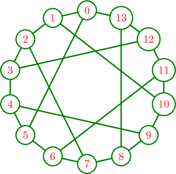
Visualizing a graph is similar to plotting functions.

sage: G = graphs.HeawoodGraph()
sage: plot(G)
Graphics object consisting of 36 graphics primitives

Defining your own graph is easy. One way is the following.

Put a vertex next to a list (recall this concept from the programming tutorial) with a colon, to show its adjacent vertices. For example, to put vertex 4 next to vertices 0 and 2, use 4:[0,2].
Now combine all these in curly braces (in the advanced appendix to the programming tutorial, this is called a dictionary ).

sage: H=Graph({0:[1,2,3], 4:[0,2], 6:[1,2,3,4,5]})
sage: plot(H)
Graphics object consisting of 18 graphics primitives

Adjacency matrices, other graphs, and similar inputs are also recognized.

Graphs have “position” information for location of vertices. There are several different ways to compute a layout, or you can compute your own. Pre-defined graphs often come with “nice” layouts.

sage: H.set_pos(H.layout_circular())
sage: plot(H)
Graphics object consisting of 18 graphics primitives

Vertices can be lots of things, for example the codewords of an error-correcting code.

Note

Technical caveat: they need to be “immutable”, like Python’s tuples.

Here we have a matrix over the integers and a matrix of variables as vertices.

sage: a=matrix([[1,2],[3,4]])
sage: var('x y z w')
(x, y, z, w)
sage: b=matrix([[x,y],[z,w]])
sage: a.set_immutable()
sage: b.set_immutable()
sage: K=DiGraph({a:[b]})
sage: show(K, vertex_size=800)

Edges can be labeled.

sage: L=graphs.CycleGraph(5)
sage: for edge in L.edges(sort=True):
....:     u = edge[0]
....:     v = edge[1]
....:     L.set_edge_label(u, v, u*v)
sage: plot(L, edge_labels=True)
Graphics object consisting of 16 graphics primitives

There are natural connections to other areas of mathematics. Here we compute the automorphism group and eigenvalues of the skeleton of a cube.

sage: C = graphs.CubeGraph(3)
sage: plot(C)
Graphics object consisting of 21 graphics primitives

sage: Aut=C.automorphism_group()
sage: print("Order of automorphism group: {}".format(Aut.order()))
Order of automorphism group:  48
sage: print("Group: \n{}".format(Aut)) # random
Group:
Permutation Group with generators [('010','100')('011','101'), ('001','010')('101','110'), ('000','001')('010','011')('100','101')('110','111')]

sage: C.spectrum()
[3, 1, 1, 1, -1, -1, -1, -3]

There is a huge amount of LaTeX support for graphs. The following graphic shows an example of what can be done; this is the Heawood graph.

$../_images/heawood-graph-latex.png$

Press ‘tab’ at the next command to see all the available options.

sage: sage.graphs.graph_latex.GraphLatex.set_option?

More Discrete Mathematics#

Discrete mathematics is a broad area, and Sage has excellent support for much of it. This is largely due to the “sage-combinat” group. These developers previously developed for MuPad (as “mupad-combinat”) but switched over to Sage shortly before MuPad was sold.

Simple Combinatorics#

Sage can work with basic combinatorial structures like combinations and permutations.

sage: pets = ['dog', 'cat', 'snake', 'spider']
sage: C=Combinations(pets)
sage: C.list()
[[], ['dog'], ['cat'], ['snake'], ['spider'], ['dog', 'cat'], ['dog', 'snake'], ['dog', 'spider'], ['cat', 'snake'], ['cat', 'spider'], ['snake', 'spider'], ['dog', 'cat', 'snake'], ['dog', 'cat', 'spider'], ['dog', 'snake', 'spider'], ['cat', 'snake', 'spider'], ['dog', 'cat', 'snake', 'spider']]

sage: for a, b in Combinations(pets, 2):
....:     print("The {} chases the {}.".format(a, b))
The dog chases the cat.
The dog chases the snake.
The dog chases the spider.
The cat chases the snake.
The cat chases the spider.
The snake chases the spider.

sage: for pair in Permutations(pets, 2):
....:     print(pair)
['dog', 'cat']
['dog', 'snake']
['dog', 'spider']
['cat', 'dog']
['cat', 'snake']
['cat', 'spider']
['snake', 'dog']
['snake', 'cat']
['snake', 'spider']
['spider', 'dog']
['spider', 'cat']
['spider', 'snake']

Of course, we often want these for numbers, and these are present as well. Some are familiar:

sage: Permutations(5).cardinality()
120

Others somewhat less so:

sage: D = Derangements([1,1,2,2,3,4,5])
sage: D.list()[:5]
[[2, 2, 1, 1, 4, 5, 3], [2, 2, 1, 1, 5, 3, 4], [2, 2, 1, 3, 1, 5, 4], [2, 2, 1, 3, 4, 5, 1], [2, 2, 1, 3, 5, 1, 4]]

And some somewhat more advanced – in this case, symmetric polynomials.

sage: s = SymmetricFunctions(QQ).schur()
sage: a = s([2,1])
sage: a.expand(3)
x0^2*x1 + x0*x1^2 + x0^2*x2 + 2*x0*x1*x2 + x1^2*x2 + x0*x2^2 + x1*x2^2

Various functions related to this are available as well.

sage: binomial(25,3)
2300

sage: multinomial(24,3,5)
589024800

sage: falling_factorial(10,4)
5040

Do you recognize this famous identity?

sage: var('k,n')
(k, n)
sage: sum(binomial(n,k),k,0,n)
2^n

Cryptography (for education)#

This is also briefly mentioned in the Number theory quickstart. Sage has a number of good pedagogical resources for cryptography.

sage: # Two objects to make/use encryption scheme
sage: #
sage: from sage.crypto.block_cipher.sdes import SimplifiedDES
sage: sdes = SimplifiedDES()
sage: bin = BinaryStrings()
sage: #
sage: # Convert English to binary
sage: #
sage: P = bin.encoding("Encrypt this using S-DES!")
sage: print("Binary plaintext:  {}\n".format(P))
sage: #
sage: # Choose a random key
sage: #
sage: K = sdes.list_to_string(sdes.random_key())
sage: print("Random key:  {}\n".format(K))
sage: #
sage: # Encrypt with Simplified DES
sage: #
sage: C = sdes(P, K, algorithm="encrypt")
sage: print("Encrypted:  {}\n".format(C))
sage: #
sage: # Decrypt for the round-trip
sage: #
sage: plaintxt = sdes(C, K, algorithm="decrypt")
sage: print("Decrypted:  {}\n".format(plaintxt))
sage: #
sage: # Verify easily
sage: #
sage: print("Verify encryption/decryption: {}".format(P == plaintxt))
Binary plaintext:  01000101011011100110001101110010011110010111000001110100001000000111010001101000011010010111001100100000011101010111001101101001011011100110011100100000010100110010110101000100010001010101001100100001

Random key:  0100000011

Encrypted:  00100001100001010011000111000110010000011011101011111011100011011111101111110111110010101000010010001101101010101000010011001010100001010111000010001101000011001001111111110100001000010000110001011000

Decrypted:  01000101011011100110001101110010011110010111000001110100001000000111010001101000011010010111001100100000011101010111001101101001011011100110011100100000010100110010110101000100010001010101001100100001

Verify encryption/decryption:  True

Coding Theory#

Here is a brief example of a linear binary code (group code).

Start with a generator matrix over $\ZZ/2\ZZ$.

sage: G = matrix(GF(2), [[1,1,1,0,0,0,0], [1,0,0,1,1,0,0], [0,1,0,1,0,1,0], [1,1,0,1,0,0,1]])
sage: C = LinearCode(G)

sage: C.is_self_dual()
False

sage: D = C.dual_code()
sage: D
[7, 3] linear code over GF(2)

sage: D.basis()
[
(1, 0, 1, 0, 1, 0, 1),
(0, 1, 1, 0, 0, 1, 1),
(0, 0, 0, 1, 1, 1, 1)
]

sage: D.permutation_automorphism_group()
Permutation Group with generators [(4,5)(6,7), (4,6)(5,7), (2,3)(6,7), (2,4)(3,5), (1,2)(5,6)]