Sage Quickstart for Statistics
This Sage quickstart tutorial was developed for the MAA PREP Workshop “Sage: Using Open-Source Mathematics Software with Undergraduates” (funding provided by NSF DUE 0817071). It is licensed under the Creative Commons Attribution-ShareAlike 3.0 license (CC BY-SA).
Basic Descriptive Statistics
Basic statistical functions are best to get from numpy and scipy.stats.
NumPy provides, for example, functions to compute the arithmetic mean and the standard deviation:
sage: import numpy as np
sage: if int(np.version.short_version[0]) > 1:
....:     _ = np.set_printoptions(legacy="1.25")
sage: np.mean([1, 2, 3, 5])
2.75

sage: np.std([1, 2, 2, 4, 5, 6, 8])  # rel to 1e-13
2.32992949004287
>>> from sage.all import *
>>> import numpy as np
>>> if int(np.version.short_version[Integer(0)]) > Integer(1):
...     _ = np.set_printoptions(legacy="1.25")
>>> np.mean([Integer(1), Integer(2), Integer(3), Integer(5)])
2.75

>>> np.std([Integer(1), Integer(2), Integer(2), Integer(4), Integer(5), Integer(6), Integer(8)])  # rel to 1e-13
2.32992949004287
SciPy offers many more functions, for example a function to compute the harmonic mean:
sage: from scipy.stats import hmean
sage: hmean([1, 2, 2, 4, 5, 6, 8])  # rel to 1e-13
2.5531914893617023
>>> from sage.all import *
>>> from scipy.stats import hmean
>>> hmean([Integer(1), Integer(2), Integer(2), Integer(4), Integer(5), Integer(6), Integer(8)])  # rel to 1e-13
2.5531914893617023
We do not recommend to use Python’s built in statistics module with Sage.
It has a known incompatibility with number types defined in Sage, see Issue #28234.
Distributions
Let’s generate a random sample from a given type of continuous distribution using native Python random generators.
We use the simplest method of generating random elements from a log normal distribution with (normal) mean 2 and \(\sigma=3\).
Notice that there is really no way around making some kind of loop.
sage: my_data = [lognormvariate(2, 3) for i in range(10)]
sage: my_data # random
[13.189347821530054, 151.28229284782799, 0.071974845847761343, 202.62181449742425, 1.9677158880100207, 71.959830176932542, 21.054742855786007, 3.9235315623286406, 4129.9880239483346, 16.41063858663054]
>>> from sage.all import *
>>> my_data = [lognormvariate(Integer(2), Integer(3)) for i in range(Integer(10))]
>>> my_data # random
[13.189347821530054, 151.28229284782799, 0.071974845847761343, 202.62181449742425, 1.9677158880100207, 71.959830176932542, 21.054742855786007, 3.9235315623286406, 4129.9880239483346, 16.41063858663054]
We can check whether the mean of the log of the data is close to 2.
sage: np.mean([log(item) for item in my_data]) # random
3.0769518857697618
>>> from sage.all import *
>>> np.mean([log(item) for item in my_data]) # random
3.0769518857697618
Here is an example using the Gnu scientific library under the hood.
Let
distbe the variable assigned to a continuous Gaussian/normal distribution with standard deviation of 3.Then we use the
.get_random_element()method ten times, adding 2 each time so that the mean is equal to 2.
sage: dist=RealDistribution('gaussian',3)
sage: my_data=[dist.get_random_element()+2 for _ in range(10)]
sage: my_data # random
[3.18196848067, -2.70878671264, 0.445500746768, 0.579932075555, -1.32546445128, 0.985799587162, 4.96649083229, -1.78785287243, -3.05866866979, 5.90786474822]
>>> from sage.all import *
>>> dist=RealDistribution('gaussian',Integer(3))
>>> my_data=[dist.get_random_element()+Integer(2) for _ in range(Integer(10))]
>>> my_data # random
[3.18196848067, -2.70878671264, 0.445500746768, 0.579932075555, -1.32546445128, 0.985799587162, 4.96649083229, -1.78785287243, -3.05866866979, 5.90786474822]
For now, it’s a little annoying to get histograms of such things directly. Here, we get a larger sampling of this distribution and plot a histogram with 10 bins.
sage: my_data2 = [dist.get_random_element()+2 for _ in range(1000)]
sage: T = stats.TimeSeries(my_data)
sage: T.plot_histogram(normalize=False,bins=10)
Graphics object consisting of 10 graphics primitives
>>> from sage.all import *
>>> my_data2 = [dist.get_random_element()+Integer(2) for _ in range(Integer(1000))]
>>> T = stats.TimeSeries(my_data)
>>> T.plot_histogram(normalize=False,bins=Integer(10))
Graphics object consisting of 10 graphics primitives
To access discrete distributions, we again use Scipy.
We have to
importthe modulescipy.stats.We use
binom_distto denote the binomial distribution with 20 trials and 5% expected failure rate.The
.pmf(x)method gives the probability of \(x\) failures, which we then plot in a bar chart for \(x\) from 0 to 20. (Don’t forget thatrange(21)means all integers from zero to twenty.)
sage: import scipy.stats
sage: binom_dist = scipy.stats.binom(20,.05)
sage: bar_chart([binom_dist.pmf(x) for x in range(21)])
Graphics object consisting of 1 graphics primitive
>>> from sage.all import *
>>> import scipy.stats
>>> binom_dist = scipy.stats.binom(Integer(20),RealNumber('.05'))
>>> bar_chart([binom_dist.pmf(x) for x in range(Integer(21))])
Graphics object consisting of 1 graphics primitive
The bar_chart function performs some of the duties of histograms.
Scipy’s statistics can do other things too. Here, we find the median (as the fiftieth percentile) of an earlier data set.
sage: scipy.stats.scoreatpercentile(my_data, 50) # random
0.51271641116183286
>>> from sage.all import *
>>> scipy.stats.scoreatpercentile(my_data, Integer(50)) # random
0.51271641116183286
The key thing to remember here is to look at the documentation!
Using R from within Sage
The R project is a leading software package for statistical analysis with widespread use in industry and academics.
There are several ways to access R; they are based on the rpy2 package.
One of the easiest is to just put
r()around things you want to make into statistical objects, and then …Use R commands via
r.method()to pass them on to Sage for further processing.
The following example of the Kruskal-Wallis test comes directly from
the examples in r.kruskal_test? in the notebook.
sage: # optional - rpy2
sage: x = r([2.9, 3.0, 2.5, 2.6, 3.2])      # normal subjects
sage: y = r([3.8, 2.7, 4.0, 2.4])           # with obstructive airway disease
sage: z = r([2.8, 3.4, 3.7, 2.2, 2.0])      # with asbestosis
sage: a = r([x,y,z])                        # make a long R vector of all the data
sage: b = r.factor(5*[1] + 4*[2] + 5*[3])   # create something for R to tell
....:                                       #   which subjects are which
sage: a; b                                  # show them
 [1] 2.9 3.0 2.5 2.6 3.2 3.8 2.7 4.0 2.4 2.8 3.4 3.7 2.2 2.0
 [1] 1 1 1 1 1 2 2 2 2 3 3 3 3 3
Levels: 1 2 3
>>> from sage.all import *
>>> # optional - rpy2
>>> x = r([RealNumber('2.9'), RealNumber('3.0'), RealNumber('2.5'), RealNumber('2.6'), RealNumber('3.2')])      # normal subjects
>>> y = r([RealNumber('3.8'), RealNumber('2.7'), RealNumber('4.0'), RealNumber('2.4')])           # with obstructive airway disease
>>> z = r([RealNumber('2.8'), RealNumber('3.4'), RealNumber('3.7'), RealNumber('2.2'), RealNumber('2.0')])      # with asbestosis
>>> a = r([x,y,z])                        # make a long R vector of all the data
>>> b = r.factor(Integer(5)*[Integer(1)] + Integer(4)*[Integer(2)] + Integer(5)*[Integer(3)])   # create something for R to tell
...                                       #   which subjects are which
>>> a; b                                  # show them
 [1] 2.9 3.0 2.5 2.6 3.2 3.8 2.7 4.0 2.4 2.8 3.4 3.7 2.2 2.0
 [1] 1 1 1 1 1 2 2 2 2 3 3 3 3 3
Levels: 1 2 3
sage: r.kruskal_test(a,b)             # do the KW test!                       # optional - rpy2
    Kruskal-Wallis rank sum test

data:  sage17 and sage33
Kruskal-Wallis chi-squared = 0.7714, df = 2, p-value = 0.68
>>> from sage.all import *
>>> r.kruskal_test(a,b)             # do the KW test!                       # optional - rpy2
    Kruskal-Wallis rank sum test

data:  sage17 and sage33
Kruskal-Wallis chi-squared = 0.7714, df = 2, p-value = 0.68
Looks like we can’t reject the null hypothesis here.
The best way to use R seriously is to simply ask each individual cell to
evaluate completely in R, using a so-called “percent directive”. Here
is a sample linear regression from John Verzani’s simpleR text.
Notice that R also uses the # symbol to indicate comments.
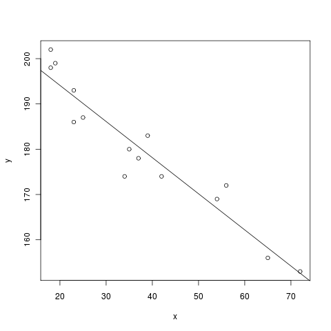
sage: %r                                                                      # optional - rpy2
....: x = c(18,23,25,35,65,54,34,56,72,19,23,42,18,39,37) # ages of individuals
....: y = c(202,186,187,180,156,169,174,172,153,199,193,174,198,183,178) # maximum heart rate of each one
....: png() # turn on plotting
....: plot(x,y) # make a plot
....: lm(y ~ x) # do the linear regression
....: abline(lm(y ~ x)) # plot the regression line
....: dev.off()     # turn off the device so it plots
Call:
lm(formula = y ~ x)

Coefficients:
(Intercept)            x
   210.0485      -0.7977

null device
          1
>>> from sage.all import *
>>> %r                                                                      # optional - rpy2
... x = c(Integer(18),Integer(23),Integer(25),Integer(35),Integer(65),Integer(54),Integer(34),Integer(56),Integer(72),Integer(19),Integer(23),Integer(42),Integer(18),Integer(39),Integer(37)) # ages of individuals
... y = c(Integer(202),Integer(186),Integer(187),Integer(180),Integer(156),Integer(169),Integer(174),Integer(172),Integer(153),Integer(199),Integer(193),Integer(174),Integer(198),Integer(183),Integer(178)) # maximum heart rate of each one
... png() # turn on plotting
... plot(x,y) # make a plot
... lm(y ~ x) # do the linear regression
... abline(lm(y ~ x)) # plot the regression line
... dev.off()     # turn off the device so it plots
Call:
lm(formula = y ~ x)

Coefficients:
(Intercept)            x
   210.0485      -0.7977

null device
          1
To get a whole worksheet to evaluate in R (and be able to ignore the
%), you could also drop down the r option in the menu close to
the top which currently has sage in it.