Static sparse graphs
What is the point ?
This class implements a Cython (di)graph structure made for efficiency. The graphs are static, i.e. no add/remove vertex/edges methods are available, nor can they easily or efficiently be implemented within this data structure.
The data structure, however, is made to save the maximum amount of computations for graph algorithms whose main operation is to list the out-neighbours of a vertex (which is precisely what BFS, DFS, distance computations and the flow-related stuff waste their life on).
The code contained in this module is written C-style. The purpose is efficiency and simplicity.
For an overview of graph data structures in sage, see
overview.
Author:
Nathann Cohen (2011)
Data structure
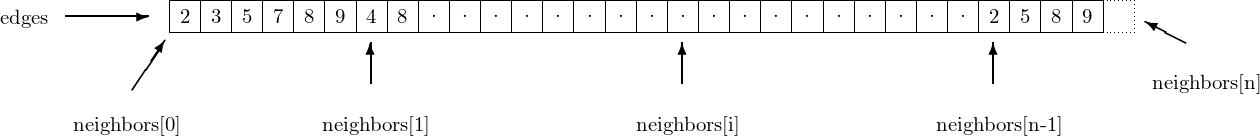
The data structure is actually pretty simple and compact. short_digraph has
five fields
n– integer; the number of vertices in the graphm– integer; the number of edges in the graphedges–uint32_t *; array whose length is the number of edges of the graphneighbors–uint32_t **; this array has size \(n+1\), and describes how the data ofedgesshould be read : the neighbors of vertex \(i\) are the elements ofedgesaddressed byneighbors[i]...neighbors[i+1]-1. The elementneighbors[n], which corresponds to no vertex (they are numbered from \(0\) to \(n-1\)) is present so that it remains easy to enumerate the neighbors of vertex \(n-1\) : the last of them is the element addressed byneighbors[n]-1. The arraysneighbors[i]are guaranteed to be sorted so the time complexity for deciding ifghas edge \((u, v)\) is \(O(\log{m})\) using binary search.edge_labels– list; this cython list associates a label to each edge of the graph. If a given edge is represented byedges[i], this its associated label can be found atedge_labels[i]. This object is usually NULL, unless the call toinit_short_digraphexplicitly requires the labels to be stored in the data structure.
In the example given above, vertex 0 has 2,3,5,7,8 and 9 as out-neighbors, but
not 4, which is an out-neighbour of vertex 1. Vertex \(n-1\) has 2, 5, 8 and 9 as
out-neighbors. neighbors[n] points toward the cell immediately after the
end of edges, hence outside of the allocated memory. It is used to
indicate the end of the outneighbors of vertex \(n-1\)
Iterating over the edges
This is the one thing to have in mind when working with this data structure:
cdef list_edges(short_digraph g):
    cdef int i, j
    for i in range(g.n):
        for j in range(g.neighbors[i+1]-g.neighbors[i]):
            print("There is an edge from {} to {}".format(i, g.neighbors[i][j]))
Advantages
Two great points :
The neighbors of a vertex are C types, and are contiguous in memory.
Storing such graphs is incredibly cheaper than storing Python structures.
Well, I think it would be hard to have anything more efficient than that to enumerate out-neighbors in sparse graphs ! :-)
Technical details
When creating a
short_digraphfrom aGraphorDiGraphnamedG, the \(i^{\text{th}}\) vertex corresponds by default tolist(G)[i]. Using optional parametervertex_list, you can specify the order of the vertices. Then \(i^{\text{th}}\) vertex will corresponds tovertex_list[i].Some methods return
bitset_tobjects when lists could be expected. There is a very usefulbitset_listfunction for this kind of problems :-)When the edges are labelled, most of the space taken by this graph is taken by edge labels. If no edge is labelled then this space is not allocated, but if any edge has a label then a (possibly empty) label is stored for each edge, which can double the memory needs.
The data structure stores the number of edges, even though it appears that this number can be reconstructed with
g.neighbors[n]-g.neighbors[0]. The trick is that not all elements of theg.edgesarray are necessarily used : when an undirected graph contains loops, only one entry of the array of size \(2m\) is used to store it, instead of the expected two. Storing the number of edges is the only way to avoid an uselessly costly computation to obtain the number of edges of an undirected, looped, AND labelled graph (think of several loops on the same vertex with different labels).The codes of this module are well documented, and many answers can be found directly in the code.
Cython functions
|
Initialize |
|
Return the number of edges in |
|
Return the out-degree of vertex \(i\) in |
|
Test the existence of an edge. |
|
Return the label associated with a given edge |
|
Allocate |
|
Initialize |
|
Free the resources used by |
Connectivity
can_be_reached_from(short_digraph g, int src, bitset_t reached)
Assuming
bitset_t reachedhas size at leastg.n, this method updatesreachedso that it represents the set of vertices that can be reached fromsrcing.
strongly_connected_component_containing_vertex(short_digraph g, short_digraph g_reversed, int v, bitset_t scc)
Assuming
bitset_t reachedhas size at leastg.n, this method updatessccso that it represents the vertices of the strongly connected component containingving. The variableg_reversedis assumed to represent the reverse ofg.
tarjan_strongly_connected_components_C(short_digraph g, int *scc)
Assuming
sccis already allocated and has size at leastg.n, this method computes the strongly connected components ofg, and outputs inscc[v]the number of the strongly connected component containingv. It returns the number of strongly connected components.
strongly_connected_components_digraph_C(short_digraph g, int nscc, int *scc, short_digraph output):
Assuming
nsccandsccare the outputs oftarjan_strongly_connected_components_Cong, this routine setsoutputto the strongly connected component digraph ofg, that is, the vertices ofoutputare the strongly connected components ofg(numbers are provided byscc), andoutputcontains an arc(C1,C2)ifghas an arc from a vertex inC1to a vertex inC2.
What is this module used for ?
It is for instance used in the sage.graphs.distances_all_pairs module,
and in the strongly_connected_components()
method.
Python functions
These functions are available so that Python modules from Sage can call the Cython routines this module implements (as they cannot directly call methods with C arguments).
- sage.graphs.base.static_sparse_graph.spectral_radius(G, prec=1e-10)[source]
Return an interval of floating point number that encloses the spectral radius of this graph
The input graph
Gmust be strongly connected.INPUT:
prec– (default:1e-10) an upper bound for the relative precision of the interval
The algorithm is iterative and uses an inequality valid for nonnegative matrices. Namely, if \(A\) is a nonnegative square matrix with Perron-Frobenius eigenvalue \(\lambda\) then the following inequality is valid for any vector \(x\)
\[\min_i \frac{(Ax)_i}{x_i} \leq \lambda \leq \max_i \frac{(Ax)_i}{x_i}\]Note
The speed of convergence of the algorithm is governed by the spectral gap (the distance to the second largest modulus of other eigenvalues). If this gap is small, then this function might not be appropriate.
The algorithm is not smart and not parallel! It uses basic interval arithmetic and native floating point arithmetic.
EXAMPLES:
sage: from sage.graphs.base.static_sparse_graph import spectral_radius

sage: G = DiGraph([(0,0),(0,1),(1,0)], loops=True)
sage: phi = (RR(1) + RR(5).sqrt() ) / 2
sage: phi  # abs tol 1e-14
1.618033988749895
sage: e_min, e_max = spectral_radius(G, 1e-14)
sage: e_min, e_max     # abs tol 1e-14
(1.618033988749894, 1.618033988749896)
sage: (e_max - e_min)  # abs tol 1e-14
1e-14
sage: e_min < phi < e_max
True
>>> from sage.all import *
>>> from sage.graphs.base.static_sparse_graph import spectral_radius

>>> G = DiGraph([(Integer(0),Integer(0)),(Integer(0),Integer(1)),(Integer(1),Integer(0))], loops=True)
>>> phi = (RR(Integer(1)) + RR(Integer(5)).sqrt() ) / Integer(2)
>>> phi  # abs tol 1e-14
1.618033988749895
>>> e_min, e_max = spectral_radius(G, RealNumber('1e-14'))
>>> e_min, e_max     # abs tol 1e-14
(1.618033988749894, 1.618033988749896)
>>> (e_max - e_min)  # abs tol 1e-14
1e-14
>>> e_min < phi < e_max
True
This function also works for graphs:
sage: G = Graph([(0,1),(0,2),(1,2),(1,3),(2,4),(3,4)])
sage: e_min, e_max = spectral_radius(G, 1e-14)
sage: e = max(G.adjacency_matrix().charpoly().roots(AA, multiplicities=False))  # needs sage.modules sage.rings.number_field
sage: e_min < e < e_max                                                         # needs sage.modules sage.rings.number_field sage.symbolic
True

sage: G.spectral_radius()  # abs tol 1e-9
(2.48119430408, 2.4811943041)
>>> from sage.all import *
>>> G = Graph([(Integer(0),Integer(1)),(Integer(0),Integer(2)),(Integer(1),Integer(2)),(Integer(1),Integer(3)),(Integer(2),Integer(4)),(Integer(3),Integer(4))])
>>> e_min, e_max = spectral_radius(G, RealNumber('1e-14'))
>>> e = max(G.adjacency_matrix().charpoly().roots(AA, multiplicities=False))  # needs sage.modules sage.rings.number_field
>>> e_min < e < e_max                                                         # needs sage.modules sage.rings.number_field sage.symbolic
True

>>> G.spectral_radius()  # abs tol 1e-9
(2.48119430408, 2.4811943041)
A larger example:
sage: # needs sage.modules
sage: G = DiGraph()
sage: G.add_edges((i,i+1) for i in range(200))
sage: G.add_edge(200,0)
sage: G.add_edge(1,0)
sage: e_min, e_max = spectral_radius(G, 0.00001)
sage: p = G.adjacency_matrix(sparse=True).charpoly()
sage: p
x^201 - x^199 - 1
sage: r = p.roots(AA, multiplicities=False)[0]                                  # needs sage.rings.number_field
sage: e_min < r < e_max                                                         # needs sage.rings.number_field
True
>>> from sage.all import *
>>> # needs sage.modules
>>> G = DiGraph()
>>> G.add_edges((i,i+Integer(1)) for i in range(Integer(200)))
>>> G.add_edge(Integer(200),Integer(0))
>>> G.add_edge(Integer(1),Integer(0))
>>> e_min, e_max = spectral_radius(G, RealNumber('0.00001'))
>>> p = G.adjacency_matrix(sparse=True).charpoly()
>>> p
x^201 - x^199 - 1
>>> r = p.roots(AA, multiplicities=False)[Integer(0)]                                  # needs sage.rings.number_field
>>> e_min < r < e_max                                                         # needs sage.rings.number_field
True
A much larger example:
sage: G = DiGraph(100000)
sage: r = list(range(100000))
sage: while not G.is_strongly_connected():
....:     shuffle(r)
....:     G.add_edges(enumerate(r), loops=False)
sage: spectral_radius(G, 1e-10)  # random  # long time
(1.9997956006500042, 1.9998043797692782)
>>> from sage.all import *
>>> G = DiGraph(Integer(100000))
>>> r = list(range(Integer(100000)))
>>> while not G.is_strongly_connected():
...     shuffle(r)
...     G.add_edges(enumerate(r), loops=False)
>>> spectral_radius(G, RealNumber('1e-10'))  # random  # long time
(1.9997956006500042, 1.9998043797692782)
The algorithm takes care of multiple edges:
sage: G = DiGraph(2,loops=True,multiedges=True)
sage: G.add_edges([(0,0),(0,0),(0,1),(1,0)])
sage: spectral_radius(G, 1e-14)  # abs tol 1e-14
(2.414213562373094, 2.414213562373095)
sage: max(G.adjacency_matrix().eigenvalues(AA))                                 # needs sage.modules sage.rings.number_field
2.414213562373095?
>>> from sage.all import *
>>> G = DiGraph(Integer(2),loops=True,multiedges=True)
>>> G.add_edges([(Integer(0),Integer(0)),(Integer(0),Integer(0)),(Integer(0),Integer(1)),(Integer(1),Integer(0))])
>>> spectral_radius(G, RealNumber('1e-14'))  # abs tol 1e-14
(2.414213562373094, 2.414213562373095)
>>> max(G.adjacency_matrix().eigenvalues(AA))                                 # needs sage.modules sage.rings.number_field
2.414213562373095?
Some bipartite graphs:
sage: G = Graph([(0,1),(0,3),(2,3)])
sage: G.spectral_radius()  # abs tol 1e-10
(1.6180339887253428, 1.6180339887592732)

sage: G = DiGraph([(0,1),(0,3),(2,3),(3,0),(1,0),(1,2)])
sage: G.spectral_radius() # abs tol 1e-10
(1.5537739740270458, 1.553773974033029)

sage: G = graphs.CompleteBipartiteGraph(1,3)
sage: G.spectral_radius()  # abs tol 1e-10
(1.7320508075688772, 1.7320508075688774)
>>> from sage.all import *
>>> G = Graph([(Integer(0),Integer(1)),(Integer(0),Integer(3)),(Integer(2),Integer(3))])
>>> G.spectral_radius()  # abs tol 1e-10
(1.6180339887253428, 1.6180339887592732)

>>> G = DiGraph([(Integer(0),Integer(1)),(Integer(0),Integer(3)),(Integer(2),Integer(3)),(Integer(3),Integer(0)),(Integer(1),Integer(0)),(Integer(1),Integer(2))])
>>> G.spectral_radius() # abs tol 1e-10
(1.5537739740270458, 1.553773974033029)

>>> G = graphs.CompleteBipartiteGraph(Integer(1),Integer(3))
>>> G.spectral_radius()  # abs tol 1e-10
(1.7320508075688772, 1.7320508075688774)
- sage.graphs.base.static_sparse_graph.strongly_connected_components_digraph(G)[source]
Return the digraph of the strongly connected components (SCCs).
This routine is used to test
strongly_connected_components_digraph_C, but it is not used by the Sage digraph. It outputs a pair[g_scc,scc], whereg_sccis the SCC digraph of g,sccis a dictionary associating to each vertexvthe number of the SCC ofv, as it appears ing_scc.EXAMPLES:
sage: from sage.graphs.base.static_sparse_graph import strongly_connected_components_digraph
sage: strongly_connected_components_digraph(digraphs.Path(3))
(Digraph on 3 vertices, {0: 2, 1: 1, 2: 0})
sage: strongly_connected_components_digraph(DiGraph(4))
(Digraph on 4 vertices, {0: 0, 1: 1, 2: 2, 3: 3})
>>> from sage.all import *
>>> from sage.graphs.base.static_sparse_graph import strongly_connected_components_digraph
>>> strongly_connected_components_digraph(digraphs.Path(Integer(3)))
(Digraph on 3 vertices, {0: 2, 1: 1, 2: 0})
>>> strongly_connected_components_digraph(DiGraph(Integer(4)))
(Digraph on 4 vertices, {0: 0, 1: 1, 2: 2, 3: 3})
- sage.graphs.base.static_sparse_graph.tarjan_strongly_connected_components(G)[source]
Return the lists of vertices in each strongly connected components (SCCs).
This method implements the Tarjan algorithm to compute the strongly connected components of the digraph. It returns a list of lists of vertices, each list of vertices representing a strongly connected component.
The basic idea of the algorithm is this: a depth-first search (DFS) begins from an arbitrary start node (and subsequent DFSes are conducted on any nodes that have not yet been found). As usual with DFSes, the search visits every node of the graph exactly once, declining to revisit any node that has already been explored. Thus, the collection of search trees is a spanning forest of the graph. The strongly connected components correspond to the subtrees of this spanning forest that have no edge directed outside the subtree.
To recover these components, during the DFS, we keep the index of a node, that is, the position in the DFS tree, and the lowlink: as soon as the subtree rooted at \(v\) has been fully explored, the lowlink of \(v\) is the smallest index reachable from \(v\) passing from descendants of \(v\). If the subtree rooted at \(v\) has been fully explored, and the index of \(v\) equals the lowlink of \(v\), that whole subtree is a new SCC.
For more information, see the Wikipedia article Tarjan%27s_strongly_connected_components_algorithm.
EXAMPLES:
sage: from sage.graphs.base.static_sparse_graph import tarjan_strongly_connected_components
sage: tarjan_strongly_connected_components(digraphs.Path(3))
[[2], [1], [0]]
sage: D = DiGraph( { 0 : [1, 3], 1 : [2], 2 : [3], 4 : [5, 6], 5 : [6] } )
sage: D.connected_components(sort=True)
[[0, 1, 2, 3], [4, 5, 6]]
sage: D = DiGraph( { 0 : [1, 3], 1 : [2], 2 : [3], 4 : [5, 6], 5 : [6] } )
sage: D.strongly_connected_components()
[[3], [2], [1], [0], [6], [5], [4]]
sage: D.add_edge([2,0])
sage: D.strongly_connected_components()
[[3], [0, 1, 2], [6], [5], [4]]
sage: D = DiGraph([('a','b'), ('b','c'), ('c', 'd'), ('d', 'b'), ('c', 'e')])
sage: [sorted(scc) for scc in D.strongly_connected_components()]
[['e'], ['b', 'c', 'd'], ['a']]
>>> from sage.all import *
>>> from sage.graphs.base.static_sparse_graph import tarjan_strongly_connected_components
>>> tarjan_strongly_connected_components(digraphs.Path(Integer(3)))
[[2], [1], [0]]
>>> D = DiGraph( { Integer(0) : [Integer(1), Integer(3)], Integer(1) : [Integer(2)], Integer(2) : [Integer(3)], Integer(4) : [Integer(5), Integer(6)], Integer(5) : [Integer(6)] } )
>>> D.connected_components(sort=True)
[[0, 1, 2, 3], [4, 5, 6]]
>>> D = DiGraph( { Integer(0) : [Integer(1), Integer(3)], Integer(1) : [Integer(2)], Integer(2) : [Integer(3)], Integer(4) : [Integer(5), Integer(6)], Integer(5) : [Integer(6)] } )
>>> D.strongly_connected_components()
[[3], [2], [1], [0], [6], [5], [4]]
>>> D.add_edge([Integer(2),Integer(0)])
>>> D.strongly_connected_components()
[[3], [0, 1, 2], [6], [5], [4]]
>>> D = DiGraph([('a','b'), ('b','c'), ('c', 'd'), ('d', 'b'), ('c', 'e')])
>>> [sorted(scc) for scc in D.strongly_connected_components()]
[['e'], ['b', 'c', 'd'], ['a']]
- sage.graphs.base.static_sparse_graph.triangles_count(G)[source]
Return the number of triangles containing \(v\), for every \(v\).
INPUT:
G– a graph
EXAMPLES:
sage: from sage.graphs.base.static_sparse_graph import triangles_count
sage: triangles_count(graphs.PetersenGraph())
{0: 0, 1: 0, 2: 0, 3: 0, 4: 0, 5: 0, 6: 0, 7: 0, 8: 0, 9: 0}
sage: sum(triangles_count(graphs.CompleteGraph(15)).values()) == 3*binomial(15,3)           # needs sage.symbolic
True
>>> from sage.all import *
>>> from sage.graphs.base.static_sparse_graph import triangles_count
>>> triangles_count(graphs.PetersenGraph())
{0: 0, 1: 0, 2: 0, 3: 0, 4: 0, 5: 0, 6: 0, 7: 0, 8: 0, 9: 0}
>>> sum(triangles_count(graphs.CompleteGraph(Integer(15))).values()) == Integer(3)*binomial(Integer(15),Integer(3))           # needs sage.symbolic
True