Young’s lattice and the RSK algorithm

This section provides some examples on Young’s lattice and the RSK (Robinson-Schensted-Knuth) algorithm explained in Chapter 8 of Stanley’s book [Stanley2013].

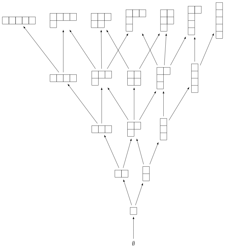
Young’s Lattice

We begin by creating the first few levels of Young’s lattice \(Y\). For this, we need to define the elements and the order relation for the poset, which is containment of partitions:

Sage

sage: level = 6
sage: elements = [b for n in range(level) for b in Partitions(n)]
sage: ord = lambda x,y: y.contains(x)
sage: Y = Poset((elements,ord), facade=True)
sage: H = Y.hasse_diagram()

Python

>>> from sage.all import *
>>> level = Integer(6)
>>> elements = [b for n in range(level) for b in Partitions(n)]
>>> ord = lambda x,y: y.contains(x)
>>> Y = Poset((elements,ord), facade=True)
>>> H = Y.hasse_diagram()

The resulting image looks best when dot2tex is installed:

Sage

sage: view(H)  # not tested

Python

>>> from sage.all import *
>>> view(H)  # not tested

We can now define the up and down operators \(U\) and \(D\) on \(\QQ Y\). First we do so on partitions, which form a basis for \(\QQ Y\):

Sage

sage: QQY = CombinatorialFreeModule(QQ,elements)

sage: def U_on_basis(la):
....:     covers = Y.upper_covers(la)
....:     return QQY.sum_of_monomials(covers)

sage: def D_on_basis(la):
....:     covers = Y.lower_covers(la)
....:     return QQY.sum_of_monomials(covers)

Python

>>> from sage.all import *
>>> QQY = CombinatorialFreeModule(QQ,elements)

>>> def U_on_basis(la):
...     covers = Y.upper_covers(la)
...     return QQY.sum_of_monomials(covers)

>>> def D_on_basis(la):
...     covers = Y.lower_covers(la)
...     return QQY.sum_of_monomials(covers)

As a shorthand, one also can write the above as:

Sage

sage: U_on_basis = QQY.sum_of_monomials * Y.upper_covers
sage: D_on_basis = QQY.sum_of_monomials * Y.lower_covers

Python

>>> from sage.all import *
>>> U_on_basis = QQY.sum_of_monomials * Y.upper_covers
>>> D_on_basis = QQY.sum_of_monomials * Y.lower_covers

Here is the result when we apply the operators to the partition \((2,1)\):

Sage

sage: la = Partition([2,1])
sage: U_on_basis(la)
B[[2, 1, 1]] + B[[2, 2]] + B[[3, 1]]
sage: D_on_basis(la)
B[[1, 1]] + B[[2]]

Python

>>> from sage.all import *
>>> la = Partition([Integer(2),Integer(1)])
>>> U_on_basis(la)
B[[2, 1, 1]] + B[[2, 2]] + B[[3, 1]]
>>> D_on_basis(la)
B[[1, 1]] + B[[2]]

Now we define the up and down operator on \(\QQ Y\):

Sage

sage: U = QQY.module_morphism(U_on_basis)
sage: D = QQY.module_morphism(D_on_basis)

Python

>>> from sage.all import *
>>> U = QQY.module_morphism(U_on_basis)
>>> D = QQY.module_morphism(D_on_basis)

We can check the identity \(D_{i+1} U_i - U_{i-1} D_i = I_i\) explicitly on all partitions of \(i=3\):

Sage

sage: for p in Partitions(3):
....:     b = QQY(p)
....:     assert D(U(b)) - U(D(b)) == b

Python

>>> from sage.all import *
>>> for p in Partitions(Integer(3)):
...     b = QQY(p)
...     assert D(U(b)) - U(D(b)) == b

We can also check that the coefficient of \(\lambda \vdash n\) in \(U^n(\emptyset)\) is equal to the number of standard Young tableaux of shape \(\lambda\):

Sage

sage: u = QQY(Partition([]))
sage: for i in range(4):
....:     u = U(u)
sage: u
B[[1, 1, 1, 1]] + 3*B[[2, 1, 1]] + 2*B[[2, 2]] + 3*B[[3, 1]] + B[[4]]

Python

>>> from sage.all import *
>>> u = QQY(Partition([]))
>>> for i in range(Integer(4)):
...     u = U(u)
>>> u
B[[1, 1, 1, 1]] + 3*B[[2, 1, 1]] + 2*B[[2, 2]] + 3*B[[3, 1]] + B[[4]]

For example, the number of standard Young tableaux of shape \((2,1,1)\) is \(3\):

Sage

sage: StandardTableaux([2,1,1]).cardinality()
3

Python

>>> from sage.all import *
>>> StandardTableaux([Integer(2),Integer(1),Integer(1)]).cardinality()
3

We can test this in general:

Sage

sage: for la in u.support():
....:     assert u[la] == StandardTableaux(la).cardinality()

Python

>>> from sage.all import *
>>> for la in u.support():
...     assert u[la] == StandardTableaux(la).cardinality()

We can also check this against the hook length formula (Theorem 8.1):

Sage

sage: def hook_length_formula(p):
....:     n = p.size()
....:     return factorial(n) // prod(p.hook_length(*c) for c in p.cells())

sage: for la in u.support():
....:     assert u[la] == hook_length_formula(la)

Python

>>> from sage.all import *
>>> def hook_length_formula(p):
...     n = p.size()
...     return factorial(n) // prod(p.hook_length(*c) for c in p.cells())

>>> for la in u.support():
...     assert u[la] == hook_length_formula(la)

RSK Algorithm

Let us now turn to the RSK algorithm. We can verify Example 8.12 as follows:

Sage

sage: p = Permutation([4,2,7,3,6,1,5])
sage: RSK(p)
[[[1, 3, 5], [2, 6], [4, 7]], [[1, 3, 5], [2, 4], [6, 7]]]

Python

>>> from sage.all import *
>>> p = Permutation([Integer(4),Integer(2),Integer(7),Integer(3),Integer(6),Integer(1),Integer(5)])
>>> RSK(p)
[[[1, 3, 5], [2, 6], [4, 7]], [[1, 3, 5], [2, 4], [6, 7]]]

The tableaux can also be displayed as tableaux:

Sage

sage: P,Q = RSK(p)
sage: P.pp()
1  3  5
2  6
4  7
sage: Q.pp()
1  3  5
2  4
6  7

Python

>>> from sage.all import *
>>> P,Q = RSK(p)
>>> P.pp()
1  3  5
2  6
4  7
>>> Q.pp()
1  3  5
2  4
6  7

The inverse RSK algorithm is implemented as follows:

Sage

sage: RSK_inverse(P,Q, output='permutation')
[4, 2, 7, 3, 6, 1, 5]

Python

>>> from sage.all import *
>>> RSK_inverse(P,Q, output='permutation')
[4, 2, 7, 3, 6, 1, 5]

We can verify that the RSK algorithm is a bijection:

Sage

sage: def check_RSK(n):
....:     for p in Permutations(n):
....:          assert RSK_inverse(*RSK(p), output='permutation') == p
sage: for n in range(5):
....:     check_RSK(n)

Python

>>> from sage.all import *
>>> def check_RSK(n):
...     for p in Permutations(n):
...          assert RSK_inverse(*RSK(p), output='permutation') == p
>>> for n in range(Integer(5)):
...     check_RSK(n)