Linear Programming (Mixed Integer)
This document explains the use of linear programming (LP) – and of mixed integer linear programming (MILP) – in Sage by illustrating it with several problems it can solve. Most of the examples given are motivated by graph-theoretic concerns, and should be understandable without any specific knowledge of this field. As a tool in Combinatorics, using linear programming amounts to understanding how to reformulate an optimization (or existence) problem through linear constraints.
This is a translation of a chapter from the book Calcul mathematique avec Sage. This book now exists in English, too.
Definition
Here we present the usual definition of what a linear program is: it is defined by a matrix \(A: \mathbb{R}^m \mapsto \mathbb{R}^n\), along with two vectors \(b,c \in \mathbb{R}^n\). Solving a linear program is searching for a vector \(x\) maximizing an objective function and satisfying a set of constraints, i.e.
where the ordering \(u \leq u'\) between two vectors means that the entries of \(u'\) are pairwise greater than the entries of \(u\). We also write:
Equivalently, we can also say that solving a linear program amounts to maximizing a linear function defined over a polytope (preimage or \(A^{-1} (\leq b)\)). These definitions, however, do not tell us how to use linear programming in combinatorics. In the following, we will show how to solve optimization problems like the Knapsack problem, the Maximum Matching problem, and a Flow problem.
Mixed integer linear programming
There are bad news coming along with this definition of linear programming: an LP can be solved in polynomial time. This is indeed bad news, because this would mean that unless we define LP of exponential size, we cannot expect LP to solve NP-complete problems, which would be a disappointment. On a brighter side, it becomes NP-complete to solve a linear program if we are allowed to specify constraints of a different kind: requiring that some variables be integers instead of real values. Such an LP is actually called a “mixed integer linear program” (some variables can be integers, some other reals). Hence, we can expect to find in the MILP framework a wide range of expressivity.
Practical
The MILP class
The MILP class in Sage represents a MILP! It is also used to
solve regular LP. It has a very small number of methods, meant to
define our set of constraints and variables, then to read the solution
found by the solvers once computed. It is also possible to export a
MILP defined with Sage to a .lp or .mps file, understood by most
solvers.
Let us ask Sage to solve the following LP:
To achieve it, we need to define a corresponding MILP object, along with 3
variables x, y and z:
sage: p = MixedIntegerLinearProgram()
sage: v = p.new_variable(real=True, nonnegative=True)
sage: x, y, z = v['x'], v['y'], v['z']
>>> from sage.all import *
>>> p = MixedIntegerLinearProgram()
>>> v = p.new_variable(real=True, nonnegative=True)
>>> x, y, z = v['x'], v['y'], v['z']
Next, we set the objective function
sage: p.set_objective(x + y + 3*z)
>>> from sage.all import *
>>> p.set_objective(x + y + Integer(3)*z)
And finally we set the constraints
sage: p.add_constraint(x + 2*y <= 4)
sage: p.add_constraint(5*z - y <= 8)
>>> from sage.all import *
>>> p.add_constraint(x + Integer(2)*y <= Integer(4))
>>> p.add_constraint(Integer(5)*z - y <= Integer(8))
The solve method returns by default the optimal value reached by
the objective function
sage: round(p.solve(), 2)
8.8
>>> from sage.all import *
>>> round(p.solve(), Integer(2))
8.8
We can read the optimal assignment found by the solver for \(x\), \(y\) and
\(z\) through the get_values method
sage: round(p.get_values(x), 2)
4.0
sage: round(p.get_values(y), 2)
0.0
sage: round(p.get_values(z), 2)
1.6
>>> from sage.all import *
>>> round(p.get_values(x), Integer(2))
4.0
>>> round(p.get_values(y), Integer(2))
0.0
>>> round(p.get_values(z), Integer(2))
1.6
Variables
In the previous example, we obtained variables through v['x'], v['y']
and v['z']. This being said, larger LP/MILP will require us to associate an
LP variable to many Sage objects, which can be integers, strings, or even the
vertices and edges of a graph. For example:
sage: x = p.new_variable(real=True, nonnegative=True)
>>> from sage.all import *
>>> x = p.new_variable(real=True, nonnegative=True)
With this new object x we can now write constraints using
x[1],...,x[15].
sage: p.add_constraint(x[1] + x[12] - x[14] >= 8)
>>> from sage.all import *
>>> p.add_constraint(x[Integer(1)] + x[Integer(12)] - x[Integer(14)] >= Integer(8))
Notice that we did not need to define the “length” of x. Actually, x
would accept any immutable object as a key, as a dictionary would. We can now
write
sage: p.add_constraint(x["I am a valid key"] +
....:                  x[("a",pi)] <= 3)
>>> from sage.all import *
>>> p.add_constraint(x["I am a valid key"] +
...                  x[("a",pi)] <= Integer(3))
And because any immutable object can be used as a key, doubly indexed variables
\(x^{1,1}, ..., x^{1,15}, x^{2,1}, ..., x^{15,15}\) can be referenced by
x[1,1],...,x[1,15],x[2,1],...,x[15,15]
sage: p.add_constraint(x[3,2] + x[5] == 6)
>>> from sage.all import *
>>> p.add_constraint(x[Integer(3),Integer(2)] + x[Integer(5)] == Integer(6))
Typed variables and bounds
Types : If you want a variable to assume only integer or binary values, use
the integer=True or binary=True arguments of the new_variable
method. Alternatively, call the set_integer and set_binary methods.
Bounds : If you want your variables to only take nonnegative values, you can
say so when calling new_variable with the argument nonnegative=True. If
you want to set a different upper/lower bound on a variable, add a constraint or
use the set_min, set_max methods.
Basic linear programs
Knapsack
The Knapsack problem is the following: given a collection of items having both a weight and a usefulness, we would like to fill a bag whose capacity is constrained while maximizing the usefulness of the items contained in the bag (we will consider the sum of the items’ usefulness). For the purpose of this tutorial, we set the restriction that the bag can only carry a certain total weight.
To achieve this, we have to associate to each object \(o\) of our
collection \(C\) a binary variable taken[o], set to 1 when the
object is in the bag, and to 0 otherwise. We are trying to solve the
following MILP
Using Sage, we will give to our items a random weight:
sage: C = 1
>>> from sage.all import *
>>> C = Integer(1)
sage: L = ["pan", "book", "knife", "gourd", "flashlight"]
>>> from sage.all import *
>>> L = ["pan", "book", "knife", "gourd", "flashlight"]
sage: L.extend(["random_stuff_" + str(i) for i in range(20)])
>>> from sage.all import *
>>> L.extend(["random_stuff_" + str(i) for i in range(Integer(20))])
sage: weight = {}
sage: usefulness = {}
>>> from sage.all import *
>>> weight = {}
>>> usefulness = {}
sage: set_random_seed(685474)
sage: for o in L:
....:     weight[o] = random()
....:     usefulness[o] = random()
>>> from sage.all import *
>>> set_random_seed(Integer(685474))
>>> for o in L:
...     weight[o] = random()
...     usefulness[o] = random()
We can now define the MILP itself
sage: p = MixedIntegerLinearProgram()
sage: taken = p.new_variable(binary=True)
>>> from sage.all import *
>>> p = MixedIntegerLinearProgram()
>>> taken = p.new_variable(binary=True)
sage: p.add_constraint(p.sum(weight[o] * taken[o] for o in L) <= C)
>>> from sage.all import *
>>> p.add_constraint(p.sum(weight[o] * taken[o] for o in L) <= C)
sage: p.set_objective(p.sum(usefulness[o] * taken[o] for o in L))
>>> from sage.all import *
>>> p.set_objective(p.sum(usefulness[o] * taken[o] for o in L))
sage: p.solve() # abs tol 1e-6
3.1502766806530307
sage: taken = p.get_values(taken)
>>> from sage.all import *
>>> p.solve() # abs tol 1e-6
3.1502766806530307
>>> taken = p.get_values(taken)
The solution found is (of course) admissible
sage: sum(weight[o] * taken[o] for o in L)  # abs tol 1e-6
0.6964959796619171
>>> from sage.all import *
>>> sum(weight[o] * taken[o] for o in L)  # abs tol 1e-6
0.6964959796619171
Should we take a flashlight?
sage: taken["flashlight"] # abs tol 1e-6
1.0
>>> from sage.all import *
>>> taken["flashlight"] # abs tol 1e-6
1.0
Wise advice. Based on purely random considerations.
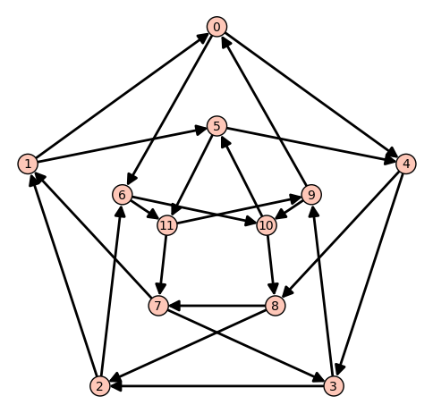
Matching
Given a graph \(G\), a matching is a set of pairwise disjoint edges. The empty set is a trivial matching. So we focus our attention on maximum matchings: we want to find in a graph a matching whose cardinality is maximal. Computing the maximum matching in a graph is a polynomial problem, which is a famous result of Edmonds. Edmonds’ algorithm is based on local improvements and the proof that a given matching is maximum if it cannot be improved. This algorithm is not the hardest to implement among those graph theory can offer, though this problem can be modeled with a very simple MILP.
To do it, we need – as previously – to associate a binary variable to each one of our objects: the edges of our graph (a value of 1 meaning that the corresponding edge is included in the maximum matching). Our constraint on the edges taken being that they are disjoint, it is enough to require that, \(x\) and \(y\) being two edges and \(m_x, m_y\) their associated variables, the inequality \(m_x + m_y \leq 1\) is satisfied, as we are sure that the two of them cannot both belong to the matching. Hence, we are able to write the MILP we want. However, the number of inequalities can be easily decreased by noticing that two edges cannot be taken simultaneously inside a matching if and only if they have a common endpoint \(v\). We can then require instead that at most one edge incident to \(v\) be taken inside the matching, which is a linear constraint. We will be solving:
Let us write the Sage code of this MILP:
sage: g = graphs.PetersenGraph()
sage: p = MixedIntegerLinearProgram()
sage: matching = p.new_variable(binary=True)
>>> from sage.all import *
>>> g = graphs.PetersenGraph()
>>> p = MixedIntegerLinearProgram()
>>> matching = p.new_variable(binary=True)
sage: p.set_objective(p.sum(matching[e] for e in g.edges(sort=False, labels=False)))
>>> from sage.all import *
>>> p.set_objective(p.sum(matching[e] for e in g.edges(sort=False, labels=False)))
sage: for v in g:
....:     p.add_constraint(p.sum(matching[e]
....:         for e in g.edges_incident(v, labels=False)) <= 1)
>>> from sage.all import *
>>> for v in g:
...     p.add_constraint(p.sum(matching[e]
...         for e in g.edges_incident(v, labels=False)) <= Integer(1))
sage: p.solve()
5.0
>>> from sage.all import *
>>> p.solve()
5.0
sage: matching = p.get_values(matching, convert=bool, tolerance=1e-3)
sage: sorted(e for e, b in matching.items() if b)   # random
[(0, 4), (1, 6), (2, 3), (5, 8), (7, 9)]
sage: len(_)
5
>>> from sage.all import *
>>> matching = p.get_values(matching, convert=bool, tolerance=RealNumber('1e-3'))
>>> sorted(e for e, b in matching.items() if b)   # random
[(0, 4), (1, 6), (2, 3), (5, 8), (7, 9)]
>>> len(_)
5
Flows
Yet another fundamental algorithm in graph theory: maximum flow! It consists, given a directed graph and two vertices \(s, t\), in sending a maximum flow from \(s\) to \(t\) using the edges of \(G\), each of them having a maximal capacity.
The definition of this problem is almost its LP formulation. We are looking for real values associated to each edge, which would represent the intensity of flow going through them, under two types of constraints:
The amount of flow arriving on a vertex (different from \(s\) or \(t\)) is equal to the amount of flow leaving it.
The amount of flow going through an edge is bounded by the capacity of this edge.
This being said, we have to maximize the amount of flow leaving \(s\): all of it will end up in \(t\), as the other vertices are sending just as much as they receive. We can model the flow problem with the following LP
We will solve the flow problem on an orientation of Chvatal’s graph, in which all the edges have a capacity of 1:
sage: g = graphs.ChvatalGraph()
sage: g = g.minimum_outdegree_orientation()
>>> from sage.all import *
>>> g = graphs.ChvatalGraph()
>>> g = g.minimum_outdegree_orientation()
sage: p = MixedIntegerLinearProgram()
sage: f = p.new_variable(real=True, nonnegative=True)
sage: s, t = 0, 2
>>> from sage.all import *
>>> p = MixedIntegerLinearProgram()
>>> f = p.new_variable(real=True, nonnegative=True)
>>> s, t = Integer(0), Integer(2)
sage: for v in g:
....:     if v != s and v != t:
....:         p.add_constraint(
....:             p.sum(f[v,u] for u in g.neighbors_out(v))
....:             - p.sum(f[u,v] for u in g.neighbors_in(v)) == 0)
>>> from sage.all import *
>>> for v in g:
...     if v != s and v != t:
...         p.add_constraint(
...             p.sum(f[v,u] for u in g.neighbors_out(v))
...             - p.sum(f[u,v] for u in g.neighbors_in(v)) == Integer(0))
sage: for e in g.edges(sort=False, labels=False):
....:     p.add_constraint(f[e] <= 1)
>>> from sage.all import *
>>> for e in g.edges(sort=False, labels=False):
...     p.add_constraint(f[e] <= Integer(1))
sage: p.set_objective(p.sum(f[s,u] for u in g.neighbors_out(s)))
>>> from sage.all import *
>>> p.set_objective(p.sum(f[s,u] for u in g.neighbors_out(s)))
sage: p.solve()  # rel tol 2e-11
2.0
>>> from sage.all import *
>>> p.solve()  # rel tol 2e-11
2.0
Solvers (backends)
Sage solves linear programs by calling specific libraries. The following libraries are currently supported:
CBC: A solver from COIN-OR, provided under the Eclipse Public License (EPL), which is an open source license but incompatible with GPL. CBC and the Sage CBC backend can be installed using the shell command:
$ sage -i -c sage_numerical_backends_coinCPLEX: Proprietary, but available for free for researchers and students through IBM’s Academic Initiative. Since Issue #27790, only versions 12.8 and above are supported.
Install CPLEX according to the instructions on the website, which includes obtaining a license key.
Then find the installation directory of your ILOG CPLEX Studio installation, which contains subdirectories
cplex,doc,opl, etc. Set the environment variableCPLEX_HOMEto this directory; for example using the following shell command (on macOS):$ export CPLEX_HOME=/Applications/CPLEX_Studio1210or (on Linux):
$ export CPLEX_HOME=/opt/ibm/ILOG/CPLEX_Studio1210Now verify that the CPLEX binary that you will find in the subdirectory
cplex/bin/ARCH-OSstarts correctly, for example:$ $CPLEX_HOME/cplex/bin/x86-64_osx/cplex Welcome to IBM(R) ILOG(R) CPLEX(R) Interactive Optimizer...
This environment variable only needs to be set for the following step: Install the Sage CPLEX backend using the shell command:
$ sage -i -c sage_numerical_backends_cplexCVXOPT: an LP solver from Python Software for Convex Optimization, uses an interior-point method, always installed in Sage.
Licensed under the GPL.
-
Licensed under the GPLv3. This solver is always installed, as the default one, in Sage.
Gurobi: Proprietary, but available for free for researchers and students via Gurobi’s Academic Program.
Install Gurobi according to the instructions on the website, which includes obtaining a license key. The installation should make the interactive Gurobi shell
gurobi.shavailable in yourPATH. Verify this by typing the shell commandgurobi.sh:$ gurobi.sh Python 3.7.4 (default, Aug 27 2019, 11:27:39) ... Gurobi Interactive Shell (mac64), Version 9.0.0 Copyright (c) 2019, Gurobi Optimization, LLC Type "help()" for help gurobi>
If this does not work, adjust your
PATHor create symbolic links so thatgurobi.shis found.Now install the Sage Gurobi backend using the shell command:
$ sage -i -c sage_numerical_backends_gurobiPPL: A solver from bugSeng.
This solver provides exact (arbitrary precision) computation, always installed in Sage.
Licensed under the GPLv3.