Affine Highest Weight Crystals
Affine highest weight crystals are infinite-dimensional. Their underlying weight lattice is the extended weight lattice including the null root \(\delta\). This is in contrast to finite-dimensional affine crystals such as for example the Kirillov-Reshetikhin crystals whose underlying weight lattice is the classical weight lattice, i.e., does not include \(\delta\).
Hence, to work with them in Sage, we need some further tools.
Littelmann path model
The Littelmann path model for highest weight crystals is implemented in Sage. It models finite highest crystals as well as affine highest weight crystals which are infinite dimensional. The elements of the crystal are piecewise linear maps in the extended weight space over \(\QQ\). For more information on the Littelmann path model, see [L1995].
Since the affine highest weight crystals are infinite, it is not possible to list all elements or draw the entire crystal graph. However, if the user is only interested in the crystal up to a certain distance or depth from the highest weight element, then one can work with the corresponding subcrystal. To view the corresponding upper part of the crystal, one can build the associated digraph:
sage: R = RootSystem(['C',3,1])
sage: La = R.weight_space(extended = True).basis()
sage: LS = crystals.LSPaths(2*La[1]); LS
The crystal of LS paths of type ['C', 3, 1] and weight 2*Lambda[1]
sage: LS.weight_lattice_realization()
Extended weight space over the Rational Field of the Root system of type ['C', 3, 1]
sage: C = LS.subcrystal(max_depth=3)
sage: sorted(C, key=str)
[(-Lambda[0] + 2*Lambda[1] - Lambda[2] + Lambda[3] - delta, Lambda[1]),
 (-Lambda[0] + Lambda[1] + Lambda[2] - delta, Lambda[0] - Lambda[1] + Lambda[2]),
 (-Lambda[0] + Lambda[1] + Lambda[2] - delta, Lambda[1]),
 (-Lambda[1] + 2*Lambda[2] - delta, Lambda[1]),
 (2*Lambda[0] - 2*Lambda[1] + 2*Lambda[2],),
 (2*Lambda[1],),
 (Lambda[0] + Lambda[2] - Lambda[3], Lambda[1]),
 (Lambda[0] - Lambda[1] + Lambda[2], Lambda[1]),
 (Lambda[0] - Lambda[2] + Lambda[3], Lambda[0] - Lambda[1] + Lambda[2]),
 (Lambda[0] - Lambda[2] + Lambda[3], Lambda[1])]

sage: G = LS.digraph(subset = C)
sage: view(G, tightpage=True)  # optional - dot2tex graphviz, not tested (opens external window)
>>> from sage.all import *
>>> R = RootSystem(['C',Integer(3),Integer(1)])
>>> La = R.weight_space(extended = True).basis()
>>> LS = crystals.LSPaths(Integer(2)*La[Integer(1)]); LS
The crystal of LS paths of type ['C', 3, 1] and weight 2*Lambda[1]
>>> LS.weight_lattice_realization()
Extended weight space over the Rational Field of the Root system of type ['C', 3, 1]
>>> C = LS.subcrystal(max_depth=Integer(3))
>>> sorted(C, key=str)
[(-Lambda[0] + 2*Lambda[1] - Lambda[2] + Lambda[3] - delta, Lambda[1]),
 (-Lambda[0] + Lambda[1] + Lambda[2] - delta, Lambda[0] - Lambda[1] + Lambda[2]),
 (-Lambda[0] + Lambda[1] + Lambda[2] - delta, Lambda[1]),
 (-Lambda[1] + 2*Lambda[2] - delta, Lambda[1]),
 (2*Lambda[0] - 2*Lambda[1] + 2*Lambda[2],),
 (2*Lambda[1],),
 (Lambda[0] + Lambda[2] - Lambda[3], Lambda[1]),
 (Lambda[0] - Lambda[1] + Lambda[2], Lambda[1]),
 (Lambda[0] - Lambda[2] + Lambda[3], Lambda[0] - Lambda[1] + Lambda[2]),
 (Lambda[0] - Lambda[2] + Lambda[3], Lambda[1])]

>>> G = LS.digraph(subset = C)
>>> view(G, tightpage=True)  # optional - dot2tex graphviz, not tested (opens external window)
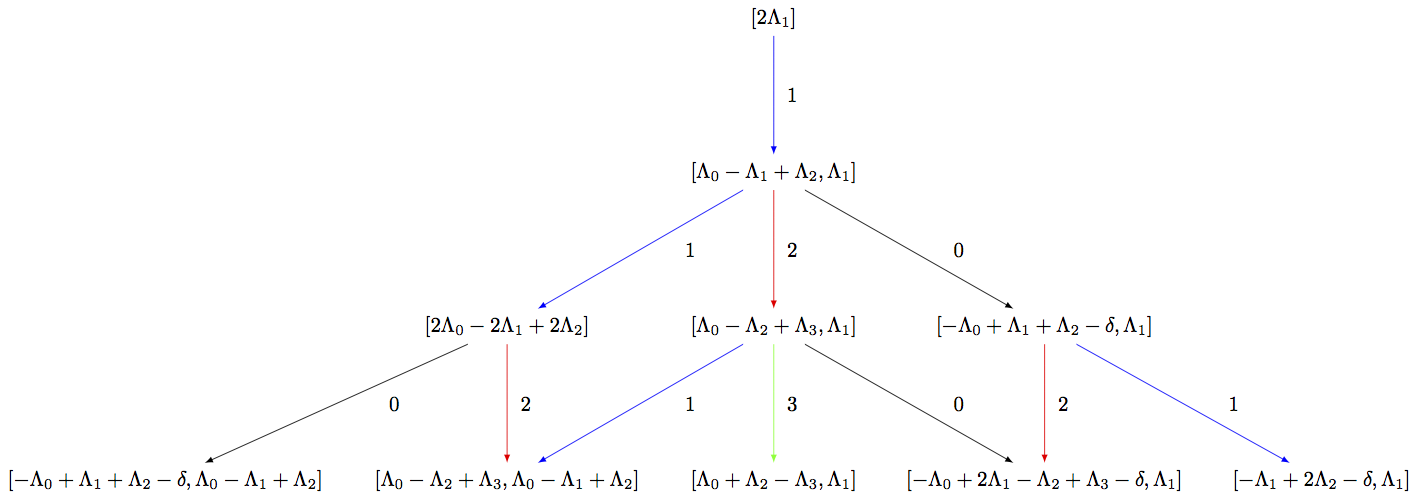
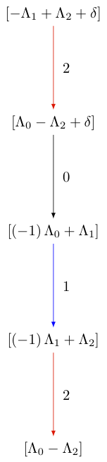
The Littelmann path model also lends itself as a model for level zero crystals which are bi-infinite. To cut out a slice of these crystals, one can use the direction option in subcrystal:
sage: R = RootSystem(['A',2,1])
sage: La = R.weight_space(extended = True).basis()
sage: LS = crystals.LSPaths(La[1]-La[0]); LS
The crystal of LS paths of type ['A', 2, 1] and weight -Lambda[0] + Lambda[1]
sage: C = LS.subcrystal(max_depth=2, direction='both')
sage: G = LS.digraph(subset = C)
sage: G.set_latex_options(edge_options=lambda uvl: ({}))
sage: view(G, tightpage=True)  # optional - dot2tex graphviz, not tested (opens external window)
>>> from sage.all import *
>>> R = RootSystem(['A',Integer(2),Integer(1)])
>>> La = R.weight_space(extended = True).basis()
>>> LS = crystals.LSPaths(La[Integer(1)]-La[Integer(0)]); LS
The crystal of LS paths of type ['A', 2, 1] and weight -Lambda[0] + Lambda[1]
>>> C = LS.subcrystal(max_depth=Integer(2), direction='both')
>>> G = LS.digraph(subset = C)
>>> G.set_latex_options(edge_options=lambda uvl: ({}))
>>> view(G, tightpage=True)  # optional - dot2tex graphviz, not tested (opens external window)
Modified Nakajima monomials
Modified Nakajima monomials have also been implemented in Sage. They model highest weight crystals in all symmetrizable types. The elements are given in terms of commuting variables \(Y_i(n)\) where \(i \in I\) and \(n \in \ZZ_{\geq 0}\). For more information on the modified Nakajima monomials, see [KKS2007].
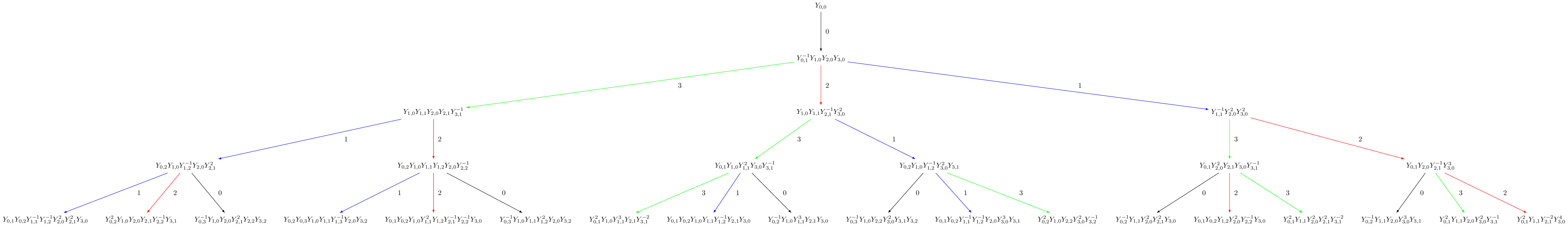
We give an example in affine type and verify that up to depth 3, it agrees with the Littelmann path model. Unlike in the LS path model, the Nakajima monomial crystals are indexed by elements in the weight lattice (rather than the weight space):
sage: La = RootSystem(['C',3,1]).weight_space(extended = True).fundamental_weights()
sage: LS = crystals.LSPaths(2*La[1]+La[2])
sage: SL = LS.subcrystal(max_depth=3)
sage: GL = LS.digraph(subset=SL)

sage: La = RootSystem(['C',3,1]).weight_lattice(extended = True).fundamental_weights()
sage: M = crystals.NakajimaMonomials(['C',3,1], 2*La[1]+La[2])
sage: SM = M.subcrystal(max_depth=3)
sage: GM = M.digraph(subset=SM)
sage: GL.is_isomorphic(GM, edge_labels=True)
True
>>> from sage.all import *
>>> La = RootSystem(['C',Integer(3),Integer(1)]).weight_space(extended = True).fundamental_weights()
>>> LS = crystals.LSPaths(Integer(2)*La[Integer(1)]+La[Integer(2)])
>>> SL = LS.subcrystal(max_depth=Integer(3))
>>> GL = LS.digraph(subset=SL)

>>> La = RootSystem(['C',Integer(3),Integer(1)]).weight_lattice(extended = True).fundamental_weights()
>>> M = crystals.NakajimaMonomials(['C',Integer(3),Integer(1)], Integer(2)*La[Integer(1)]+La[Integer(2)])
>>> SM = M.subcrystal(max_depth=Integer(3))
>>> GM = M.digraph(subset=SM)
>>> GL.is_isomorphic(GM, edge_labels=True)
True
Now we do an example of a simply-laced (and hence symmetrizable) hyperbolic type \(H_1^{(4)}\), which comes from the complete graph on 4 vertices:
sage: CM = CartanMatrix([[2, -1, -1,-1],[-1,2,-1,-1],[-1,-1,2,-1],[-1,-1,-1,2]]); CM
[ 2 -1 -1 -1]
[-1  2 -1 -1]
[-1 -1  2 -1]
[-1 -1 -1  2]
sage: La = RootSystem(CM).weight_lattice().fundamental_weights()
sage: M = crystals.NakajimaMonomials(CM, La[0])
sage: SM = M.subcrystal(max_depth=4)
sage: GM = M.digraph(subset=SM) # long time
>>> from sage.all import *
>>> CM = CartanMatrix([[Integer(2), -Integer(1), -Integer(1),-Integer(1)],[-Integer(1),Integer(2),-Integer(1),-Integer(1)],[-Integer(1),-Integer(1),Integer(2),-Integer(1)],[-Integer(1),-Integer(1),-Integer(1),Integer(2)]]); CM
[ 2 -1 -1 -1]
[-1  2 -1 -1]
[-1 -1  2 -1]
[-1 -1 -1  2]
>>> La = RootSystem(CM).weight_lattice().fundamental_weights()
>>> M = crystals.NakajimaMonomials(CM, La[Integer(0)])
>>> SM = M.subcrystal(max_depth=Integer(4))
>>> GM = M.digraph(subset=SM) # long time