Walks in graphs
This section provides some examples on Chapter 1 of Stanley’s book [Stanley2013].
We begin by creating a graph with 4 vertices:
sage: G = Graph(4)
sage: G
Graph on 4 vertices
>>> from sage.all import *
>>> G = Graph(Integer(4))
>>> G
Graph on 4 vertices
This graph has no edges yet:
sage: G.vertices(sort=True)
[0, 1, 2, 3]
sage: G.edges(sort=True)
[]
>>> from sage.all import *
>>> G.vertices(sort=True)
[0, 1, 2, 3]
>>> G.edges(sort=True)
[]
Before we can add edges, we need to tell Sage that our graph can have loops and multiple edges.:
sage: G.allow_loops(True)
sage: G.allow_multiple_edges(True)
>>> from sage.all import *
>>> G.allow_loops(True)
>>> G.allow_multiple_edges(True)
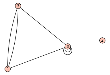
Now we are ready to add our edges by specifying a tuple of vertices that are connected by an edge. If there are multiple edges, we need to add the tuple with multiplicity.:
sage: G.add_edges([(0,0),(0,0),(0,1),(0,3),(1,3),(1,3)])
>>> from sage.all import *
>>> G.add_edges([(Integer(0),Integer(0)),(Integer(0),Integer(0)),(Integer(0),Integer(1)),(Integer(0),Integer(3)),(Integer(1),Integer(3)),(Integer(1),Integer(3))])
Now let us look at the graph!
sage: G.plot()
Graphics object consisting of 11 graphics primitives
>>> from sage.all import *
>>> G.plot()
Graphics object consisting of 11 graphics primitives

We can construct the adjacency matrix:
sage: A = G.adjacency_matrix()
sage: A
[2 1 0 1]
[1 0 0 2]
[0 0 0 0]
[1 2 0 0]
>>> from sage.all import *
>>> A = G.adjacency_matrix()
>>> A
[2 1 0 1]
[1 0 0 2]
[0 0 0 0]
[1 2 0 0]
The entry in row \(i\) and column \(j\) of the \(\ell\)-th power of \(A\) gives us the number of paths of length \(\ell\) from vertex \(i\) to vertex \(j\). Let us verify this:
sage: A**2
[6 4 0 4]
[4 5 0 1]
[0 0 0 0]
[4 1 0 5]
>>> from sage.all import *
>>> A**Integer(2)
[6 4 0 4]
[4 5 0 1]
[0 0 0 0]
[4 1 0 5]
There are 4 paths of length 2 from vertex \(0\) to vertex \(1\): take either loop at \(0\) and then the edge \((0, 1)\) (2 choices) or take the edge \((0, 3)\) and then either of the two edges \((3, 1)\) (two choices):
sage: (A**2)[0,1]
4
>>> from sage.all import *
>>> (A**Integer(2))[Integer(0),Integer(1)]
4
To count the number of closed walks, we can also look at the sum of the \(\ell\)-th powers of the eigenvalues. Even though the eigenvalues are not integers, we find that the sum of their squares is an integer:
sage: A.eigenvalues()
[0, -2, 0.5857864376269049?, 3.414213562373095?]
sage: sum(la**2 for la in A.eigenvalues())
16.00000000000000?
>>> from sage.all import *
>>> A.eigenvalues()
[0, -2, 0.5857864376269049?, 3.414213562373095?]
>>> sum(la**Integer(2) for la in A.eigenvalues())
16.00000000000000?
We can achieve the same by looking at the trace of the \(\ell\)-th power of the matrix:
sage: (A**2).trace()
16
>>> from sage.all import *
>>> (A**Integer(2)).trace()
16