Affine Finite Crystals

In this document we briefly explain the construction and implementation of the Kirillov–Reshetikhin crystals of [FourierEtAl2009].

Kirillov–Reshetikhin (KR) crystals are finite-dimensional affine crystals corresponding to Kirillov–Reshektikhin modules. They were first conjectured to exist in [HatayamaEtAl2001]. The proof of their existence for nonexceptional types was given in [OkadoSchilling2008] and their combinatorial models were constructed in [FourierEtAl2009]. Kirillov-Reshetikhin crystals $B^{r,s}$ are indexed first by their type (like $A_n^{(1)}$, $B_n^{(1)}$, …) with underlying index set $I=\{0,1,\dots ,n\}$ and two integers $r$ and $s$. The integers $s$ only needs to satisfy $s>0$, whereas $r$ is a node of the finite Dynkin diagram $r\in I\setminus \{0\}$.

Their construction relies on several cases which we discuss separately. In all cases when removing the zero arrows, the crystal decomposes as a (direct sum of) classical crystals which gives the crystal structure for the index set $I_0=\{1,2,\dots ,n\}$. Then the zero arrows are added by either exploiting a symmetry of the Dynkin diagram or by using embeddings of crystals.

Type $A_n^{(1)}$

The Dynkin diagram for affine type $A$ has a rotational symmetry mapping $\sigma :i\mapsto i+1$ where we view the indices modulo $n+1$:

Sage

sage: C = CartanType(['A',3,1])
sage: C.dynkin_diagram()
0
O-------+
|       |
|       |
O---O---O
1   2   3
A3~

Python

>>> from sage.all import *
>>> C = CartanType(['A',Integer(3),Integer(1)])
>>> C.dynkin_diagram()
0
O-------+
|       |
|       |
O---O---O
1   2   3
A3~

The classical decomposition of $B^{r,s}$ is the $A_n$ highest weight crystal $B(s{\omega }_r)$ or equivalently the crystal of tableaux labelled by the rectangular partition $(s^r)$:

$$B^{r,s}\cong B(s{\omega }_r)\text{as a }\{1,2,\dots ,n\}\text{-crystal}$$

In Sage we can see this via:

Sage

sage: K = crystals.KirillovReshetikhin(['A',3,1],1,1)
sage: K.classical_decomposition()
The crystal of tableaux of type ['A', 3] and shape(s) [[1]]
sage: K.list()
[[[1]], [[2]], [[3]], [[4]]]

sage: K = crystals.KirillovReshetikhin(['A',3,1],2,1)
sage: K.classical_decomposition()
The crystal of tableaux of type ['A', 3] and shape(s) [[1, 1]]

Python

>>> from sage.all import *
>>> K = crystals.KirillovReshetikhin(['A',Integer(3),Integer(1)],Integer(1),Integer(1))
>>> K.classical_decomposition()
The crystal of tableaux of type ['A', 3] and shape(s) [[1]]
>>> K.list()
[[[1]], [[2]], [[3]], [[4]]]

>>> K = crystals.KirillovReshetikhin(['A',Integer(3),Integer(1)],Integer(2),Integer(1))
>>> K.classical_decomposition()
The crystal of tableaux of type ['A', 3] and shape(s) [[1, 1]]

One can change between the classical and affine crystal using the methods lift and retract:

Sage

sage: K = crystals.KirillovReshetikhin(['A',3,1],2,1)
sage: b = K(rows=[[1],[3]]); type(b)
<class 'sage.combinat.crystals.kirillov_reshetikhin.KR_type_A_with_category.element_class'>
sage: b.lift()
[[1], [3]]
sage: type(b.lift())
<class 'sage.combinat.crystals.tensor_product.CrystalOfTableaux_with_category.element_class'>

sage: b = crystals.Tableaux(['A',3], shape = [1,1])(rows=[[1],[3]])
sage: K.retract(b)
[[1], [3]]
sage: type(K.retract(b))
<class 'sage.combinat.crystals.kirillov_reshetikhin.KR_type_A_with_category.element_class'>

Python

>>> from sage.all import *
>>> K = crystals.KirillovReshetikhin(['A',Integer(3),Integer(1)],Integer(2),Integer(1))
>>> b = K(rows=[[Integer(1)],[Integer(3)]]); type(b)
<class 'sage.combinat.crystals.kirillov_reshetikhin.KR_type_A_with_category.element_class'>
>>> b.lift()
[[1], [3]]
>>> type(b.lift())
<class 'sage.combinat.crystals.tensor_product.CrystalOfTableaux_with_category.element_class'>

>>> b = crystals.Tableaux(['A',Integer(3)], shape = [Integer(1),Integer(1)])(rows=[[Integer(1)],[Integer(3)]])
>>> K.retract(b)
[[1], [3]]
>>> type(K.retract(b))
<class 'sage.combinat.crystals.kirillov_reshetikhin.KR_type_A_with_category.element_class'>

The $0$-arrows are obtained using the analogue of $\sigma$, called the promotion operator $\mathrm{pr}$, on the level of crystals via:

$$\begin{array}{r}\begin{array}{c}{f}_0={\mathrm{pr}}^{-1}\circ f_1\circ \mathrm{pr}\\ e_0={\mathrm{pr}}^{-1}\circ e_1\circ \mathrm{pr}\end{array}\end{array}$$

In Sage this can be achieved as follows:

Sage

sage: K = crystals.KirillovReshetikhin(['A',3,1],2,1)
sage: b = K.module_generator(); b
[[1], [2]]
sage: b.f(0)
sage: b.e(0)
[[2], [4]]

sage: K.promotion()(b.lift())
[[2], [3]]
sage: K.promotion()(b.lift()).e(1)
[[1], [3]]
sage: K.promotion_inverse()(K.promotion()(b.lift()).e(1))
[[2], [4]]

Python

>>> from sage.all import *
>>> K = crystals.KirillovReshetikhin(['A',Integer(3),Integer(1)],Integer(2),Integer(1))
>>> b = K.module_generator(); b
[[1], [2]]
>>> b.f(Integer(0))
>>> b.e(Integer(0))
[[2], [4]]

>>> K.promotion()(b.lift())
[[2], [3]]
>>> K.promotion()(b.lift()).e(Integer(1))
[[1], [3]]
>>> K.promotion_inverse()(K.promotion()(b.lift()).e(Integer(1)))
[[2], [4]]

KR crystals are level $0$ crystals, meaning that the weight of all elements in these crystals is zero:

Sage

sage: K = crystals.KirillovReshetikhin(['A',3,1],2,1)
sage: b = K.module_generator(); b.weight()
-Lambda[0] + Lambda[2]
sage: b.weight().level()
0

Python

>>> from sage.all import *
>>> K = crystals.KirillovReshetikhin(['A',Integer(3),Integer(1)],Integer(2),Integer(1))
>>> b = K.module_generator(); b.weight()
-Lambda[0] + Lambda[2]
>>> b.weight().level()
0

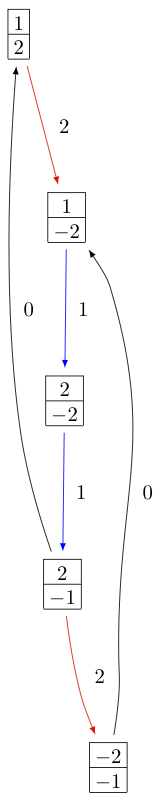
The KR crystal $B^{1,1}$ of type $A_2^{(1)}$ looks as follows:

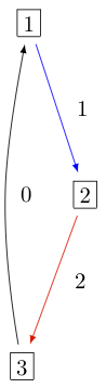
In Sage this can be obtained via:

Sage

sage: K = crystals.KirillovReshetikhin(['A',2,1],1,1)
sage: G = K.digraph()
sage: view(G, tightpage=True) # optional - dot2tex graphviz, not tested (opens external window)

Python

>>> from sage.all import *
>>> K = crystals.KirillovReshetikhin(['A',Integer(2),Integer(1)],Integer(1),Integer(1))
>>> G = K.digraph()
>>> view(G, tightpage=True) # optional - dot2tex graphviz, not tested (opens external window)

Types $D_n^{(1)}$, $B_n^{(1)}$, $A_{2n-1}^{(2)}$

The Dynkin diagrams for types $D_n^{(1)}$, $B_n^{(1)}$, $A_{2n-1}^{(2)}$ are invariant under interchanging nodes $0$ and $1$:

Sage

sage: n = 5
sage: C = CartanType(['D',n,1]); C.dynkin_diagram()
  0 O   O 5
    |   |
    |   |
O---O---O---O
1   2   3   4
D5~
sage: C = CartanType(['B',n,1]); C.dynkin_diagram()
    O 0
    |
    |
O---O---O---O=>=O
1   2   3   4   5
B5~
sage: C = CartanType(['A',2*n-1,2]); C.dynkin_diagram()
    O 0
    |
    |
O---O---O---O=<=O
1   2   3   4   5
B5~*

Python

>>> from sage.all import *
>>> n = Integer(5)
>>> C = CartanType(['D',n,Integer(1)]); C.dynkin_diagram()
  0 O   O 5
    |   |
    |   |
O---O---O---O
1   2   3   4
D5~
>>> C = CartanType(['B',n,Integer(1)]); C.dynkin_diagram()
    O 0
    |
    |
O---O---O---O=>=O
1   2   3   4   5
B5~
>>> C = CartanType(['A',Integer(2)*n-Integer(1),Integer(2)]); C.dynkin_diagram()
    O 0
    |
    |
O---O---O---O=<=O
1   2   3   4   5
B5~*

The underlying classical algebras obtained when removing node $0$ are type ${\mathfrak{g}}_0=D_n,B_n,C_n$, respectively. The classical decomposition into a ${\mathfrak{g}}_0$ crystal is a direct sum:

$$B^{r,s}\cong \underset{\lambda }{⨁}B(\lambda )\text{as a }\{1,2,\dots ,n\}\text{-crystal}$$

where $\lambda$ is obtained from $s{\omega }_r$ (or equivalently a rectangular partition of shape $(s^r)$) by removing vertical dominoes. This in fact only holds in the ranges $1\le r\le n-2$ for type $D_n^{(1)}$, and $1\le r\le n$ for types $B_n^{(1)}$ and $A_{2n-1}^{(2)}$:

Sage

sage: K = crystals.KirillovReshetikhin(['D',6,1],4,2)
sage: K.classical_decomposition()
The crystal of tableaux of type ['D', 6] and shape(s)
 [[], [1, 1], [1, 1, 1, 1], [2, 2], [2, 2, 1, 1], [2, 2, 2, 2]]

Python

>>> from sage.all import *
>>> K = crystals.KirillovReshetikhin(['D',Integer(6),Integer(1)],Integer(4),Integer(2))
>>> K.classical_decomposition()
The crystal of tableaux of type ['D', 6] and shape(s)
 [[], [1, 1], [1, 1, 1, 1], [2, 2], [2, 2, 1, 1], [2, 2, 2, 2]]

For type $B_n^{(1)}$ and $r=n$, one needs to be aware that ${\omega }_n$ is a spin weight and hence corresponds in the partition language to a column of height $n$ and width $1/2$:

Sage

sage: K = crystals.KirillovReshetikhin(['B',3,1],3,1)
sage: K.classical_decomposition()
The crystal of tableaux of type ['B', 3] and shape(s) [[1/2, 1/2, 1/2]]

Python

>>> from sage.all import *
>>> K = crystals.KirillovReshetikhin(['B',Integer(3),Integer(1)],Integer(3),Integer(1))
>>> K.classical_decomposition()
The crystal of tableaux of type ['B', 3] and shape(s) [[1/2, 1/2, 1/2]]

As for type $A_n^{(1)}$, the Dynkin automorphism induces a promotion-type operator $\sigma$ on the level of crystals. In this case in can however happen that the automorphism changes between classical components:

Sage

sage: K = crystals.KirillovReshetikhin(['D',4,1],2,1)
sage: b = K.module_generator(); b
[[1], [2]]
sage: K.automorphism(b)
[[2], [-1]]
sage: b = K(rows=[[2],[-2]])
sage: K.automorphism(b)
[]

Python

>>> from sage.all import *
>>> K = crystals.KirillovReshetikhin(['D',Integer(4),Integer(1)],Integer(2),Integer(1))
>>> b = K.module_generator(); b
[[1], [2]]
>>> K.automorphism(b)
[[2], [-1]]
>>> b = K(rows=[[Integer(2)],[-Integer(2)]])
>>> K.automorphism(b)
[]

This operator $\sigma$ is used to define the affine crystal operators:

$$\begin{array}{r}\begin{array}{c}{f}_0=\sigma \circ f_1\circ \sigma \\ e_0=\sigma \circ e_1\circ \sigma \end{array}\end{array}$$

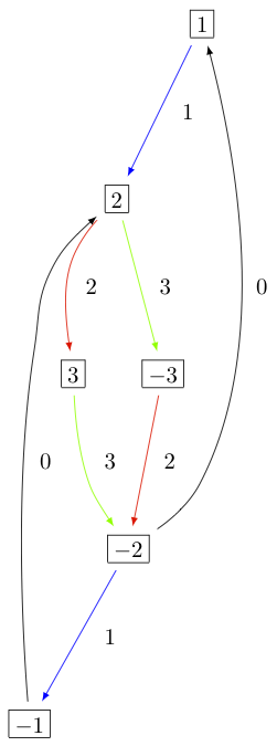
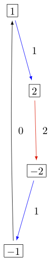
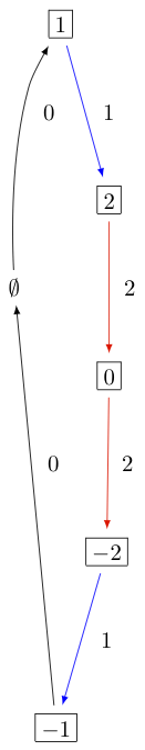
The KR crystals $B^{1,1}$ of types $D_3^{(1)}$, $B_2^{(1)}$, and $A_5^{(2)}$ are, respectively:

Type $C_n^{(1)}$

The Dynkin diagram of type $C_n^{(1)}$ has a symmetry $\sigma (i)=n-i$:

Sage

sage: C = CartanType(['C',4,1]); C.dynkin_diagram()
O=>=O---O---O=<=O
0   1   2   3   4
C4~

Python

>>> from sage.all import *
>>> C = CartanType(['C',Integer(4),Integer(1)]); C.dynkin_diagram()
O=>=O---O---O=<=O
0   1   2   3   4
C4~

The classical subalgebra when removing the 0 node is of type $C_n$.

However, in this case the crystal $B^{r,s}$ is not constructed using $\sigma$, but rather using a virtual crystal construction. $B^{r,s}$ of type $C_n^{(1)}$ is realized inside ${\hat{V}}^{r,s}$ of type $A_{2n+1}^{(2)}$ using:

$$\begin{array}{r}\begin{array}{c}{e}_0={\hat{e}}_0{\hat{e}}_1\text{and}{e}_i={\hat{e}}_{i+1}\text{for}1\le i\le n\\ f_0={\hat{f}}_0{\hat{f}}_1\text{and}{f}_i={\hat{f}}_{i+1}\text{for}1\le i\le n\end{array}\end{array}$$

where ${\hat{e}}_i$ and ${\hat{f}}_i$ are the crystal operator in the ambient crystal ${\hat{V}}^{r,s}$:

Sage

sage: K = crystals.KirillovReshetikhin(['C',3,1],1,2); K.ambient_crystal()
Kirillov-Reshetikhin crystal of type ['B', 4, 1]^* with (r,s)=(1,2)

Python

>>> from sage.all import *
>>> K = crystals.KirillovReshetikhin(['C',Integer(3),Integer(1)],Integer(1),Integer(2)); K.ambient_crystal()
Kirillov-Reshetikhin crystal of type ['B', 4, 1]^* with (r,s)=(1,2)

The classical decomposition for $1\le r<n$ is given by:

$$B^{r,s}\cong \underset{\lambda }{⨁}B(\lambda )\text{as a }\{1,2,\dots ,n\}\text{-crystal}$$

where $\lambda$ is obtained from $s{\omega }_r$ (or equivalently a rectangular partition of shape $(s^r)$) by removing horizontal dominoes:

Sage

sage: K = crystals.KirillovReshetikhin(['C',3,1],2,4)
sage: K.classical_decomposition()
The crystal of tableaux of type ['C', 3] and shape(s) [[], [2], [4], [2, 2], [4, 2], [4, 4]]

Python

>>> from sage.all import *
>>> K = crystals.KirillovReshetikhin(['C',Integer(3),Integer(1)],Integer(2),Integer(4))
>>> K.classical_decomposition()
The crystal of tableaux of type ['C', 3] and shape(s) [[], [2], [4], [2, 2], [4, 2], [4, 4]]

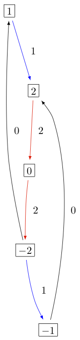
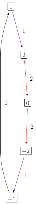
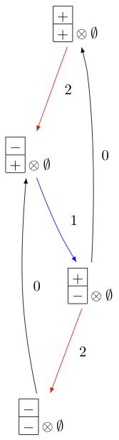
The KR crystal $B^{1,1}$ of type $C_2^{(1)}$ looks as follows:

Types $D_{n+1}^{(2)}$, $A_{2n}^{(2)}$

The Dynkin diagrams of types $D_{n+1}^{(2)}$ and $A_{2n}^{(2)}$ look as follows:

Sage

sage: C = CartanType(['D',5,2]); C.dynkin_diagram()
O=<=O---O---O=>=O
0   1   2   3   4
C4~*

sage: C = CartanType(['A',8,2]); C.dynkin_diagram()
O=<=O---O---O=<=O
0   1   2   3   4
BC4~

Python

>>> from sage.all import *
>>> C = CartanType(['D',Integer(5),Integer(2)]); C.dynkin_diagram()
O=<=O---O---O=>=O
0   1   2   3   4
C4~*

>>> C = CartanType(['A',Integer(8),Integer(2)]); C.dynkin_diagram()
O=<=O---O---O=<=O
0   1   2   3   4
BC4~

The classical subdiagram is of type $B_n$ for type $D_{n+1}^{(2)}$ and of type $C_n$ for type $A_{2n}^{(2)}$. The classical decomposition for these KR crystals for $1\le r<n$ for type $D_{n+1}^{(2)}$ and $1\le r\le n$ for type $A_{2n}^{(2)}$ is given by:

$$B^{r,s}\cong \underset{\lambda }{⨁}B(\lambda )\text{as a }\{1,2,\dots ,n\}\text{-crystal}$$

where $\lambda$ is obtained from $s{\omega }_r$ (or equivalently a rectangular partition of shape $(s^r)$) by removing single boxes:

Sage

sage: K = crystals.KirillovReshetikhin(['D',5,2],2,2)
sage: K.classical_decomposition()
The crystal of tableaux of type ['B', 4] and shape(s) [[], [1], [2], [1, 1], [2, 1], [2, 2]]

sage: K = crystals.KirillovReshetikhin(['A',8,2],2,2)
sage: K.classical_decomposition()
The crystal of tableaux of type ['C', 4] and shape(s) [[], [1], [2], [1, 1], [2, 1], [2, 2]]

Python

>>> from sage.all import *
>>> K = crystals.KirillovReshetikhin(['D',Integer(5),Integer(2)],Integer(2),Integer(2))
>>> K.classical_decomposition()
The crystal of tableaux of type ['B', 4] and shape(s) [[], [1], [2], [1, 1], [2, 1], [2, 2]]

>>> K = crystals.KirillovReshetikhin(['A',Integer(8),Integer(2)],Integer(2),Integer(2))
>>> K.classical_decomposition()
The crystal of tableaux of type ['C', 4] and shape(s) [[], [1], [2], [1, 1], [2, 1], [2, 2]]

The KR crystals are constructed using an injective map into a KR crystal of type $C_n^{(1)}$

$$S:B^{r,s}\to B_{C_n^{(1)}}^{r,2s}\text{such that }S(e_{i}b)=e_i^{m_i}S(b)\text{ and }S(f_{i}b)=f_i^{m_i}S(b)$$

where

$$(m_0,\dots ,m_n)=(1,2,\dots ,2,1)\text{ for type }{D}_{n+1}^{(2)}\text{and}(1,2,\dots ,2,2)\text{ for type }{A}_{2n}^{(2)}.$$

Sage

sage: K = crystals.KirillovReshetikhin(['D',5,2],1,2); K.ambient_crystal()
Kirillov-Reshetikhin crystal of type ['C', 4, 1] with (r,s)=(1,4)
sage: K = crystals.KirillovReshetikhin(['A',8,2],1,2); K.ambient_crystal()
Kirillov-Reshetikhin crystal of type ['C', 4, 1] with (r,s)=(1,4)

Python

>>> from sage.all import *
>>> K = crystals.KirillovReshetikhin(['D',Integer(5),Integer(2)],Integer(1),Integer(2)); K.ambient_crystal()
Kirillov-Reshetikhin crystal of type ['C', 4, 1] with (r,s)=(1,4)
>>> K = crystals.KirillovReshetikhin(['A',Integer(8),Integer(2)],Integer(1),Integer(2)); K.ambient_crystal()
Kirillov-Reshetikhin crystal of type ['C', 4, 1] with (r,s)=(1,4)

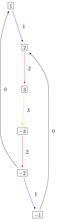
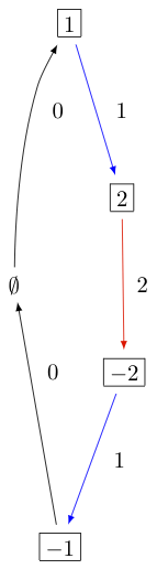
The KR crystals $B^{1,1}$ of type $D_3^{(2)}$ and $A_4^{(2)}$ look as follows:

As you can see from the Dynkin diagram for type $A_{2n}^{(2)}$, mapping the nodes $i\mapsto n-i$ yields the same diagram, but with relabelled nodes. In this case the classical subdiagram is of type $B_n$ instead of $C_n$. One can also construct the KR crystal $B^{r,s}$ of type $A_{2n}^{(2)}$ based on this classical decomposition. In this case the classical decomposition is the sum over all weights obtained from $s{\omega }_r$ by removing horizontal dominoes:

Sage

sage: C = CartanType(['A',6,2]).dual()
sage: Kdual = crystals.KirillovReshetikhin(C,2,2)
sage: Kdual.classical_decomposition()
The crystal of tableaux of type ['B', 3] and shape(s) [[], [2], [2, 2]]

Python

>>> from sage.all import *
>>> C = CartanType(['A',Integer(6),Integer(2)]).dual()
>>> Kdual = crystals.KirillovReshetikhin(C,Integer(2),Integer(2))
>>> Kdual.classical_decomposition()
The crystal of tableaux of type ['B', 3] and shape(s) [[], [2], [2, 2]]

Looking at the picture, one can see that this implementation is isomorphic to the other implementation based on the $C_n$ decomposition up to a relabeling of the arrows:

Sage

sage: C = CartanType(['A',4,2])
sage: K = crystals.KirillovReshetikhin(C,1,1)
sage: Kdual = crystals.KirillovReshetikhin(C.dual(),1,1)
sage: G = K.digraph()
sage: Gdual = Kdual.digraph()
sage: f = { 1:1, 0:2, 2:0 }
sage: for u,v,label in Gdual.edges(sort=False):
....:     Gdual.set_edge_label(u,v,f[label])
sage: G.is_isomorphic(Gdual, edge_labels = True)
True

Python

>>> from sage.all import *
>>> C = CartanType(['A',Integer(4),Integer(2)])
>>> K = crystals.KirillovReshetikhin(C,Integer(1),Integer(1))
>>> Kdual = crystals.KirillovReshetikhin(C.dual(),Integer(1),Integer(1))
>>> G = K.digraph()
>>> Gdual = Kdual.digraph()
>>> f = { Integer(1):Integer(1), Integer(0):Integer(2), Integer(2):Integer(0) }
>>> for u,v,label in Gdual.edges(sort=False):
...     Gdual.set_edge_label(u,v,f[label])
>>> G.is_isomorphic(Gdual, edge_labels = True)
True

Exceptional nodes

The KR crystals $B^{n,s}$ for types $C_n^{(1)}$ and $D_{n+1}^{(2)}$ were excluded from the above discussion. They are associated to the exceptional node $r=n$ and in this case the classical decomposition is irreducible:

$$B^{n,s}\cong B(s{\omega }_n).$$

In Sage:

Sage

sage: K = crystals.KirillovReshetikhin(['C',2,1],2,1)
sage: K.classical_decomposition()
The crystal of tableaux of type ['C', 2] and shape(s) [[1, 1]]

sage: K = crystals.KirillovReshetikhin(['D',3,2],2,1)
sage: K.classical_decomposition()
The crystal of tableaux of type ['B', 2] and shape(s) [[1/2, 1/2]]

Python

>>> from sage.all import *
>>> K = crystals.KirillovReshetikhin(['C',Integer(2),Integer(1)],Integer(2),Integer(1))
>>> K.classical_decomposition()
The crystal of tableaux of type ['C', 2] and shape(s) [[1, 1]]

>>> K = crystals.KirillovReshetikhin(['D',Integer(3),Integer(2)],Integer(2),Integer(1))
>>> K.classical_decomposition()
The crystal of tableaux of type ['B', 2] and shape(s) [[1/2, 1/2]]

The KR crystals $B^{n,s}$ and $B^{n-1,s}$ of type $D_n^{(1)}$ are also special. They decompose as:

$$B^{n,s}\cong B(s{\omega }_n)\text{ and }{B}^{n-1,s}\cong B(s{\omega }_{n-1}).$$

Sage

sage: K = crystals.KirillovReshetikhin(['D',4,1],4,1)
sage: K.classical_decomposition()
The crystal of tableaux of type ['D', 4] and shape(s) [[1/2, 1/2, 1/2, 1/2]]
sage: K = crystals.KirillovReshetikhin(['D',4,1],3,1)
sage: K.classical_decomposition()
The crystal of tableaux of type ['D', 4] and shape(s) [[1/2, 1/2, 1/2, -1/2]]

Python

>>> from sage.all import *
>>> K = crystals.KirillovReshetikhin(['D',Integer(4),Integer(1)],Integer(4),Integer(1))
>>> K.classical_decomposition()
The crystal of tableaux of type ['D', 4] and shape(s) [[1/2, 1/2, 1/2, 1/2]]
>>> K = crystals.KirillovReshetikhin(['D',Integer(4),Integer(1)],Integer(3),Integer(1))
>>> K.classical_decomposition()
The crystal of tableaux of type ['D', 4] and shape(s) [[1/2, 1/2, 1/2, -1/2]]

Type $E_6^{(1)}$

In [JonesEtAl2010] the KR crystals $B^{r,s}$ for $r=1,2,6$ in type $E_6^{(1)}$ were constructed exploiting again a Dynkin diagram automorphism, namely the automorphism $\sigma$ of order 3 which maps $0\mapsto 1\mapsto 6\mapsto 0$:

Sage

sage: C = CartanType(['E',6,1]); C.dynkin_diagram()
        O 0
        |
        |
        O 2
        |
        |
O---O---O---O---O
1   3   4   5   6
E6~

Python

>>> from sage.all import *
>>> C = CartanType(['E',Integer(6),Integer(1)]); C.dynkin_diagram()
        O 0
        |
        |
        O 2
        |
        |
O---O---O---O---O
1   3   4   5   6
E6~

The crystals $B^{1,s}$ and $B^{6,s}$ are irreducible as classical crystals:

Sage

sage: K = crystals.KirillovReshetikhin(['E',6,1],1,1)
sage: K.classical_decomposition()
Direct sum of the crystals Family (Finite dimensional highest weight crystal of type ['E', 6] and highest weight Lambda[1],)
sage: K = crystals.KirillovReshetikhin(['E',6,1],6,1)
sage: K.classical_decomposition()
Direct sum of the crystals Family (Finite dimensional highest weight crystal of type ['E', 6] and highest weight Lambda[6],)

Python

>>> from sage.all import *
>>> K = crystals.KirillovReshetikhin(['E',Integer(6),Integer(1)],Integer(1),Integer(1))
>>> K.classical_decomposition()
Direct sum of the crystals Family (Finite dimensional highest weight crystal of type ['E', 6] and highest weight Lambda[1],)
>>> K = crystals.KirillovReshetikhin(['E',Integer(6),Integer(1)],Integer(6),Integer(1))
>>> K.classical_decomposition()
Direct sum of the crystals Family (Finite dimensional highest weight crystal of type ['E', 6] and highest weight Lambda[6],)

whereas for the adjoint node $r=2$ we have the decomposition

$$B^{2,s}\cong \underset{k=0}{\overset{s}{⨁}}B(k{\omega }_2)$$

Sage

sage: K = crystals.KirillovReshetikhin(['E',6,1],2,1)
sage: K.classical_decomposition()
Direct sum of the crystals Family (Finite dimensional highest weight crystal of type ['E', 6] and highest weight 0,
Finite dimensional highest weight crystal of type ['E', 6] and highest weight Lambda[2])

Python

>>> from sage.all import *
>>> K = crystals.KirillovReshetikhin(['E',Integer(6),Integer(1)],Integer(2),Integer(1))
>>> K.classical_decomposition()
Direct sum of the crystals Family (Finite dimensional highest weight crystal of type ['E', 6] and highest weight 0,
Finite dimensional highest weight crystal of type ['E', 6] and highest weight Lambda[2])

The promotion operator on the crystal corresponding to $\sigma$ can be calculated explicitly:

Sage

sage: K = crystals.KirillovReshetikhin(['E',6,1],1,1)
sage: promotion = K.promotion()
sage: u = K.module_generator(); u
[(1,)]
sage: promotion(u.lift())
[(-1, 6)]

Python

>>> from sage.all import *
>>> K = crystals.KirillovReshetikhin(['E',Integer(6),Integer(1)],Integer(1),Integer(1))
>>> promotion = K.promotion()
>>> u = K.module_generator(); u
[(1,)]
>>> promotion(u.lift())
[(-1, 6)]

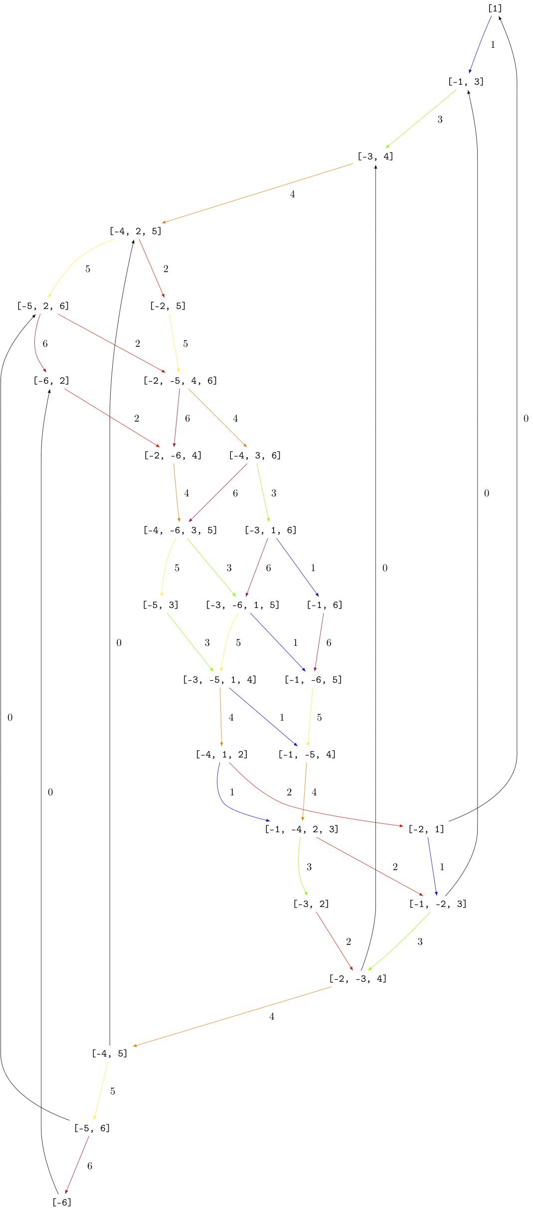
The crystal $B^{1,1}$ is already of dimension 27. The elements $b$ of this crystal are labelled by tuples which specify their nonzero ${\varphi }_i(b)$ and ${ϵ}_i(b)$. For example, $[-6,2]$ indicates that ${\varphi }_2([-6,2])={ϵ}_6([-6,2])=1$ and all others are equal to zero:

Sage

sage: K = crystals.KirillovReshetikhin(['E',6,1],1,1)
sage: K.cardinality()
27

Python

>>> from sage.all import *
>>> K = crystals.KirillovReshetikhin(['E',Integer(6),Integer(1)],Integer(1),Integer(1))
>>> K.cardinality()
27

Single column KR crystals

A single column KR crystal is $B^{r,1}$ for any $r\in I_0$.

In [LNSSS14I] and [LNSSS14II], it was shown that single column KR crystals can be constructed by projecting level 0 crystals of LS paths onto the classical weight lattice. We first verify that we do get an isomorphic crystal for $B^{1,1}$ in type $E_6^{(1)}$:

Sage

sage: K = crystals.KirillovReshetikhin(['E',6,1], 1,1)
sage: K2 = crystals.kirillov_reshetikhin.LSPaths(['E',6,1], 1,1)
sage: K.digraph().is_isomorphic(K2.digraph(), edge_labels=True)
True

Python

>>> from sage.all import *
>>> K = crystals.KirillovReshetikhin(['E',Integer(6),Integer(1)], Integer(1),Integer(1))
>>> K2 = crystals.kirillov_reshetikhin.LSPaths(['E',Integer(6),Integer(1)], Integer(1),Integer(1))
>>> K.digraph().is_isomorphic(K2.digraph(), edge_labels=True)
True

Here is an example in $E_8^{(1)}$ and we calculate its classical decomposition:

Sage

sage: K = crystals.kirillov_reshetikhin.LSPaths(['E',8,1], 8,1)
sage: K.cardinality()
249
sage: L = [x for x in K if x.is_highest_weight([1,2,3,4,5,6,7,8])]
sage: [x.weight() for x in L]
[-2*Lambda[0] + Lambda[8], 0]

Python

>>> from sage.all import *
>>> K = crystals.kirillov_reshetikhin.LSPaths(['E',Integer(8),Integer(1)], Integer(8),Integer(1))
>>> K.cardinality()
249
>>> L = [x for x in K if x.is_highest_weight([Integer(1),Integer(2),Integer(3),Integer(4),Integer(5),Integer(6),Integer(7),Integer(8)])]
>>> [x.weight() for x in L]
[-2*Lambda[0] + Lambda[8], 0]

Applications

An important notion for finite-dimensional affine crystals is perfectness. The crucial property is that a crystal $B$ is perfect of level $\ell$ if there is a bijection between level $\ell$ dominant weights and elements in

$$B_{\min }=\{b\in B\mid \mathrm{lev}(\phi (b))=\ell \}.$$

For a precise definition of perfect crystals see [HongKang2002] . In [FourierEtAl2010] it was proven that for the nonexceptional types $B^{r,s}$ is perfect as long as $s/c_r$ is an integer. Here $c_r=1$ except $c_r=2$ for $1\le r<n$ in type $C_n^{(1)}$ and $r=n$ in type $B_n^{(1)}$.

Here we verify this using Sage for $B^{1,1}$ of type $C_3^{(1)}$:

Sage

sage: K = crystals.KirillovReshetikhin(['C',3,1],1,1)
sage: Lambda = K.weight_lattice_realization().fundamental_weights(); Lambda
Finite family {0: Lambda[0], 1: Lambda[1], 2: Lambda[2], 3: Lambda[3]}
sage: [w.level() for w in Lambda]
[1, 1, 1, 1]
sage: Bmin = [b for b in K if b.Phi().level() == 1 ]; Bmin
[[[1]], [[2]], [[3]], [[-3]], [[-2]], [[-1]]]
sage: [b.Phi() for b in Bmin]
[Lambda[1], Lambda[2], Lambda[3], Lambda[2], Lambda[1], Lambda[0]]

Python

>>> from sage.all import *
>>> K = crystals.KirillovReshetikhin(['C',Integer(3),Integer(1)],Integer(1),Integer(1))
>>> Lambda = K.weight_lattice_realization().fundamental_weights(); Lambda
Finite family {0: Lambda[0], 1: Lambda[1], 2: Lambda[2], 3: Lambda[3]}
>>> [w.level() for w in Lambda]
[1, 1, 1, 1]
>>> Bmin = [b for b in K if b.Phi().level() == Integer(1) ]; Bmin
[[[1]], [[2]], [[3]], [[-3]], [[-2]], [[-1]]]
>>> [b.Phi() for b in Bmin]
[Lambda[1], Lambda[2], Lambda[3], Lambda[2], Lambda[1], Lambda[0]]

As you can see, both $b=1$ and $b=-2$ satisfy $\phi (b)={\mathrm{\Lambda }}_1$. Hence there is no bijection between the minimal elements in $B_{\min }$ and level 1 weights. Therefore, $B^{1,1}$ of type $C_3^{(1)}$ is not perfect. However, $B^{1,2}$ of type $C_n^{(1)}$ is a perfect crystal:

Sage

sage: K = crystals.KirillovReshetikhin(['C',3,1],1,2)
sage: Lambda = K.weight_lattice_realization().fundamental_weights()
sage: Bmin = [b for b in K if b.Phi().level() == 1 ]
sage: [b.Phi() for b in Bmin]
[Lambda[0], Lambda[3], Lambda[2], Lambda[1]]

Python

>>> from sage.all import *
>>> K = crystals.KirillovReshetikhin(['C',Integer(3),Integer(1)],Integer(1),Integer(2))
>>> Lambda = K.weight_lattice_realization().fundamental_weights()
>>> Bmin = [b for b in K if b.Phi().level() == Integer(1) ]
>>> [b.Phi() for b in Bmin]
[Lambda[0], Lambda[3], Lambda[2], Lambda[1]]

Perfect crystals can be used to construct infinite-dimensional highest weight crystals and Demazure crystals using the Kyoto path model [KKMMNN1992]. We construct Example 10.6.5 in [HongKang2002]:

Sage

sage: K = crystals.KirillovReshetikhin(['A',1,1], 1,1)
sage: La = RootSystem(['A',1,1]).weight_lattice().fundamental_weights()
sage: B = crystals.KyotoPathModel(K, La[0])
sage: B.highest_weight_vector()
[[[2]]]

sage: K = crystals.KirillovReshetikhin(['A',2,1], 1,1)
sage: La = RootSystem(['A',2,1]).weight_lattice().fundamental_weights()
sage: B = crystals.KyotoPathModel(K, La[0])
sage: B.highest_weight_vector()
[[[3]]]

sage: K = crystals.KirillovReshetikhin(['C',2,1], 2,1)
sage: La = RootSystem(['C',2,1]).weight_lattice().fundamental_weights()
sage: B = crystals.KyotoPathModel(K, La[1])
sage: B.highest_weight_vector()
[[[2], [-2]]]

Python

>>> from sage.all import *
>>> K = crystals.KirillovReshetikhin(['A',Integer(1),Integer(1)], Integer(1),Integer(1))
>>> La = RootSystem(['A',Integer(1),Integer(1)]).weight_lattice().fundamental_weights()
>>> B = crystals.KyotoPathModel(K, La[Integer(0)])
>>> B.highest_weight_vector()
[[[2]]]

>>> K = crystals.KirillovReshetikhin(['A',Integer(2),Integer(1)], Integer(1),Integer(1))
>>> La = RootSystem(['A',Integer(2),Integer(1)]).weight_lattice().fundamental_weights()
>>> B = crystals.KyotoPathModel(K, La[Integer(0)])
>>> B.highest_weight_vector()
[[[3]]]

>>> K = crystals.KirillovReshetikhin(['C',Integer(2),Integer(1)], Integer(2),Integer(1))
>>> La = RootSystem(['C',Integer(2),Integer(1)]).weight_lattice().fundamental_weights()
>>> B = crystals.KyotoPathModel(K, La[Integer(1)])
>>> B.highest_weight_vector()
[[[2], [-2]]]

Energy function and one-dimensional configuration sum

For tensor products of Kirillov-Reshehtikhin crystals, there also exists the important notion of the energy function. It can be defined as the sum of certain local energy functions and the $R$-matrix. In Theorem 7.5 in [SchillingTingley2011] it was shown that for perfect crystals of the same level the energy $D(b)$ is the same as the affine grading (up to a normalization). The affine grading is defined as the minimal number of applications of $e_0$ to $b$ to reach a ground state path. Computationally, this algorithm is a lot more efficient than the computation involving the $R$-matrix and has been implemented in Sage:

Sage

sage: K = crystals.KirillovReshetikhin(['A',2,1],1,1)
sage: T = crystals.TensorProduct(K,K,K)
sage: hw = [b for b in T if all(b.epsilon(i)==0 for i in [1,2])]
sage: for b in hw:
....:     print("{} {}".format(b, b.energy_function()))
[[[1]], [[1]], [[1]]] 0
[[[1]], [[2]], [[1]]] 2
[[[2]], [[1]], [[1]]] 1
[[[3]], [[2]], [[1]]] 3

Python

>>> from sage.all import *
>>> K = crystals.KirillovReshetikhin(['A',Integer(2),Integer(1)],Integer(1),Integer(1))
>>> T = crystals.TensorProduct(K,K,K)
>>> hw = [b for b in T if all(b.epsilon(i)==Integer(0) for i in [Integer(1),Integer(2)])]
>>> for b in hw:
...     print("{} {}".format(b, b.energy_function()))
[[[1]], [[1]], [[1]]] 0
[[[1]], [[2]], [[1]]] 2
[[[2]], [[1]], [[1]]] 1
[[[3]], [[2]], [[1]]] 3

The affine grading can be computed even for nonperfect crystals:

Sage

sage: K = crystals.KirillovReshetikhin(['C',4,1],1,2)
sage: K1 = crystals.KirillovReshetikhin(['C',4,1],1,1)
sage: T = crystals.TensorProduct(K,K1)
sage: hw = [b for b in T if all(b.epsilon(i)==0 for i in [1,2,3,4])]
sage: for b in hw:
....:     print("{} {}".format(b, b.affine_grading()))
[[], [[1]]] 1
[[[1, 1]], [[1]]] 2
[[[1, 2]], [[1]]] 1
[[[1, -1]], [[1]]] 0

Python

>>> from sage.all import *
>>> K = crystals.KirillovReshetikhin(['C',Integer(4),Integer(1)],Integer(1),Integer(2))
>>> K1 = crystals.KirillovReshetikhin(['C',Integer(4),Integer(1)],Integer(1),Integer(1))
>>> T = crystals.TensorProduct(K,K1)
>>> hw = [b for b in T if all(b.epsilon(i)==Integer(0) for i in [Integer(1),Integer(2),Integer(3),Integer(4)])]
>>> for b in hw:
...     print("{} {}".format(b, b.affine_grading()))
[[], [[1]]] 1
[[[1, 1]], [[1]]] 2
[[[1, 2]], [[1]]] 1
[[[1, -1]], [[1]]] 0

The one-dimensional configuration sum of a crystal $B$ is the graded sum by energy of the weight of all elements $b\in B$:

$$X(B)=\sum _{b\in B}{x}^{\mathrm{weight}(b)}{q}^{D(b)}$$

Here is an example of how you can compute the one-dimensional configuration sum in Sage:

Sage

sage: K = crystals.KirillovReshetikhin(['A',2,1],1,1)
sage: T = crystals.TensorProduct(K,K)
sage: T.one_dimensional_configuration_sum()
B[-2*Lambda[1] + 2*Lambda[2]] + (q+1)*B[-Lambda[1]]
 + (q+1)*B[Lambda[1] - Lambda[2]] + B[2*Lambda[1]]
 + B[-2*Lambda[2]] + (q+1)*B[Lambda[2]]

Python

>>> from sage.all import *
>>> K = crystals.KirillovReshetikhin(['A',Integer(2),Integer(1)],Integer(1),Integer(1))
>>> T = crystals.TensorProduct(K,K)
>>> T.one_dimensional_configuration_sum()
B[-2*Lambda[1] + 2*Lambda[2]] + (q+1)*B[-Lambda[1]]
 + (q+1)*B[Lambda[1] - Lambda[2]] + B[2*Lambda[1]]
 + B[-2*Lambda[2]] + (q+1)*B[Lambda[2]]