Fusion Rings

class sage.algebras.fusion_rings.fusion_ring.FusionRing(ct, base_ring=Integer Ring, prefix=None, style='lattice', k=None, conjugate=False, cyclotomic_order=None, fusion_labels=None, inject_variables=False)

Bases: WeylCharacterRing

Return the Fusion Ring (Verlinde Algebra) of level k.

INPUT:

• ct – the Cartan type of a simple (finite-dimensional) Lie algebra

• k – nonnegative integer

• conjugate – (default: False) set True to obtain the complex conjugate ring

• cyclotomic_order – (default: computed depending on ct and k)

• fusion_labels – (default: None) either a tuple of strings to use as labels of the basis of simple objects, or a string from which the labels will be constructed

• inject_variables – (default: False) use with fusion_labels. If inject_variables is True, the fusion labels will be variables that can be accessed from the command line

The cyclotomic order is an integer \(N\) such that all computations will return elements of the cyclotomic field of \(N\)-th roots of unity. Normally you will never need to change this but consider changing it if root_of_unity() raises a ValueError.

This algebra has a basis (sometimes called primary fields but here called simple objects) indexed by the weights of level \(\leq k\). These arise as the fusion algebras of Wess-Zumino-Witten (WZW) conformal field theories, or as Grothendieck groups of tilting modules for quantum groups at roots of unity. The FusionRing class is implemented as a variant of the WeylCharacterRing.

REFERENCES:

• [BaKi2001] Chapter 3

• [DFMS1996] Chapter 16

• [EGNO2015] Chapter 8

• [Feingold2004]

• [Fuchs1994]

• [Row2006]

• [Walton1990]

• [Wan2010]

EXAMPLES:

Sage

sage: A22 = FusionRing("A2", 2)
sage: [f1, f2] = A22.fundamental_weights()
sage: M = [A22(x) for x in [0*f1, 2*f1, 2*f2, f1+f2, f2, f1]]
sage: [M[3] * x for x in M]
[A22(1,1),
 A22(0,1),
 A22(1,0),
 A22(0,0) + A22(1,1),
 A22(0,1) + A22(2,0),
 A22(1,0) + A22(0,2)]

Python

>>> from sage.all import *
>>> A22 = FusionRing("A2", Integer(2))
>>> [f1, f2] = A22.fundamental_weights()
>>> M = [A22(x) for x in [Integer(0)*f1, Integer(2)*f1, Integer(2)*f2, f1+f2, f2, f1]]
>>> [M[Integer(3)] * x for x in M]
[A22(1,1),
 A22(0,1),
 A22(1,0),
 A22(0,0) + A22(1,1),
 A22(0,1) + A22(2,0),
 A22(1,0) + A22(0,2)]

You may assign your own labels to the basis elements. In the next example, we create the \(SO(5)\) fusion ring of level \(2\), check the weights of the basis elements, then assign new labels to them while injecting them into the global namespace:

Sage

sage: B22 = FusionRing("B2", 2)
sage: b = [B22(x) for x in B22.get_order()]; b
[B22(0,0), B22(1,0), B22(0,1), B22(2,0), B22(1,1), B22(0,2)]
sage: [x.weight() for x in b]
[(0, 0), (1, 0), (1/2, 1/2), (2, 0), (3/2, 1/2), (1, 1)]
sage: B22.fusion_labels(['I0', 'Y1', 'X', 'Z', 'Xp', 'Y2'], inject_variables=True)
sage: b = [B22(x) for x in B22.get_order()]; b
[I0, Y1, X, Z, Xp, Y2]
sage: [(x, x.weight()) for x in b]
[(I0, (0, 0)),
 (Y1, (1, 0)),
 (X, (1/2, 1/2)),
 (Z, (2, 0)),
 (Xp, (3/2, 1/2)),
 (Y2, (1, 1))]
sage: X * Y1
X + Xp
sage: Z * Z
I0

Python

>>> from sage.all import *
>>> B22 = FusionRing("B2", Integer(2))
>>> b = [B22(x) for x in B22.get_order()]; b
[B22(0,0), B22(1,0), B22(0,1), B22(2,0), B22(1,1), B22(0,2)]
>>> [x.weight() for x in b]
[(0, 0), (1, 0), (1/2, 1/2), (2, 0), (3/2, 1/2), (1, 1)]
>>> B22.fusion_labels(['I0', 'Y1', 'X', 'Z', 'Xp', 'Y2'], inject_variables=True)
>>> b = [B22(x) for x in B22.get_order()]; b
[I0, Y1, X, Z, Xp, Y2]
>>> [(x, x.weight()) for x in b]
[(I0, (0, 0)),
 (Y1, (1, 0)),
 (X, (1/2, 1/2)),
 (Z, (2, 0)),
 (Xp, (3/2, 1/2)),
 (Y2, (1, 1))]
>>> X * Y1
X + Xp
>>> Z * Z
I0

A fixed order of the basis keys is available with get_order(). This is the order used by methods such as s_matrix(). You may use CombinatorialFreeModule.set_order() to reorder the basis:

Sage

sage: B22.set_order([x.weight() for x in [I0, Y1, Y2, X, Xp, Z]])
sage: [B22(x) for x in B22.get_order()]
[I0, Y1, Y2, X, Xp, Z]

Python

>>> from sage.all import *
>>> B22.set_order([x.weight() for x in [I0, Y1, Y2, X, Xp, Z]])
>>> [B22(x) for x in B22.get_order()]
[I0, Y1, Y2, X, Xp, Z]

To reset the labels, you may run fusion_labels() with no parameter:

Sage

sage: B22.fusion_labels()
sage: [B22(x) for x in B22.get_order()]
[B22(0,0), B22(1,0), B22(0,2), B22(0,1), B22(1,1), B22(2,0)]

Python

>>> from sage.all import *
>>> B22.fusion_labels()
>>> [B22(x) for x in B22.get_order()]
[B22(0,0), B22(1,0), B22(0,2), B22(0,1), B22(1,1), B22(2,0)]

To reset the order to the default, simply set it to the list of basis element keys:

Sage

sage: B22.set_order(B22.basis().keys().list())
sage: [B22(x) for x in B22.get_order()]
[B22(0,0), B22(1,0), B22(0,1), B22(2,0), B22(1,1), B22(0,2)]

Python

>>> from sage.all import *
>>> B22.set_order(B22.basis().keys().list())
>>> [B22(x) for x in B22.get_order()]
[B22(0,0), B22(1,0), B22(0,1), B22(2,0), B22(1,1), B22(0,2)]

The fusion ring has a number of methods that reflect its role as the Grothendieck ring of a modular tensor category (MTC). These include twist methods Element.twist() and Element.ribbon() for its elements related to the ribbon structure, and the \(S\)-matrix s_ij().

There are two natural normalizations of the \(S\)-matrix. Both are explained in Chapter 3 of [BaKi2001]. The one that is computed by the method s_matrix(), or whose individual entries are computed by s_ij() is denoted \(\tilde{s}\) in [BaKi2001]. It is not unitary.

The unitary \(S\)-matrix is \(s=D^{-1/2}\tilde{s}\) where

\[D = \sum_V d_i(V)^2.\]

The sum is over all simple objects \(V\) with \(d_i(V)\) the quantum dimension. We will call quantity \(D\) the global quantum dimension and \(\sqrt{D}\) the total quantum order. They are computed by global_q_dimension() and total_q_order(). The unitary \(S\)-matrix \(s\) may be obtained using s_matrix() with the option unitary=True.

Let us check the Verlinde formula, which is [DFMS1996] (16.3). This famous identity states that

\[N^k_{ij} = \sum_l \frac{s(i, \ell)\, s(j, \ell)\, \overline{s(k, \ell)}}{s(I, \ell)},\]

where \(N^k_{ij}\) are the fusion coefficients, i.e. the structure constants of the fusion ring, and I is the unit object. The \(S\)-matrix has the property that if \(i*\) denotes the dual object of \(i\), implemented in Sage as i.dual(), then

\[s(i*, j) = s(i, j*) = \overline{s(i, j)}.\]

This is equation (16.5) in [DFMS1996]. Thus with \(N_{ijk}=N^{k*}_{ij}\) the Verlinde formula is equivalent to

\[N_{ijk} = \sum_l \frac{s(i, \ell)\, s(j, \ell)\, s(k, \ell)}{s(I, \ell)},\]

In this formula \(s\) is the normalized unitary \(S\)-matrix denoted \(s\) in [BaKi2001]. We may define a function that corresponds to the right-hand side, except using \(\tilde{s}\) instead of \(s\):

Sage

sage: def V(i, j, k):
....:     R = i.parent()
....:     return sum(R.s_ij(i, l) * R.s_ij(j, l) * R.s_ij(k, l) / R.s_ij(R.one(), l)
....:                for l in R.basis())

Python

>>> from sage.all import *
>>> def V(i, j, k):
...     R = i.parent()
...     return sum(R.s_ij(i, l) * R.s_ij(j, l) * R.s_ij(k, l) / R.s_ij(R.one(), l)
...                for l in R.basis())

This does not produce self.N_ijk(i, j, k) exactly, because of the missing normalization factor. The following code to check the Verlinde formula takes this into account:

Sage

sage: def test_verlinde(R):
....:     b0 = R.one()
....:     c = R.global_q_dimension()
....:     return all(V(i, j, k) == c * R.N_ijk(i, j, k) for i in R.basis()
....:                for j in R.basis() for k in R.basis())

Python

>>> from sage.all import *
>>> def test_verlinde(R):
...     b0 = R.one()
...     c = R.global_q_dimension()
...     return all(V(i, j, k) == c * R.N_ijk(i, j, k) for i in R.basis()
...                for j in R.basis() for k in R.basis())

Every fusion ring should pass this test:

Sage

sage: test_verlinde(FusionRing("A2", 1))
True
sage: test_verlinde(FusionRing("B4", 2)) # long time (.56s)
True

Python

>>> from sage.all import *
>>> test_verlinde(FusionRing("A2", Integer(1)))
True
>>> test_verlinde(FusionRing("B4", Integer(2))) # long time (.56s)
True

As an exercise, the reader may verify the examples in Section 5.3 of [RoStWa2009]. Here we check the example of the Ising modular tensor category, which is related to the Belavin, Polyakov, Zamolodchikov minimal model \(M(4, 3)\) or to an \(E_8\) coset model. See [DFMS1996] Sections 7.4.2 and 18.4.1. [RoStWa2009] Example 5.3.4 tells us how to construct it as the conjugate of the \(E_8\) level 2 FusionRing:

Sage

sage: I = FusionRing("E8", 2, conjugate=True)
sage: I.fusion_labels(["i0", "p", "s"], inject_variables=True)
sage: b = I.basis().list(); b
[i0, p, s]
sage: Matrix([[x*y for x in b] for y in b]) # long time (.93s)
[    i0      p      s]
[     p     i0      s]
[     s      s i0 + p]
sage: [x.twist() for x in b]
[0, 1, 1/8]
sage: [x.ribbon() for x in b]
[1, -1, zeta128^8]
sage: [I.r_matrix(i, j, k) for (i, j, k) in [(s, s, i0), (p, p, i0), (p, s, s), (s, p, s), (s, s, p)]]
[-zeta128^56, -1, -zeta128^32, -zeta128^32, zeta128^24]
sage: I.r_matrix(s, s, i0) == I.root_of_unity(-1/8)
True
sage: I.global_q_dimension()
4
sage: I.total_q_order()
2
sage: [x.q_dimension()^2 for x in b]
[1, 1, 2]
sage: I.s_matrix()
[                       1                        1 -zeta128^48 + zeta128^16]
[                       1                        1  zeta128^48 - zeta128^16]
[-zeta128^48 + zeta128^16  zeta128^48 - zeta128^16                        0]
sage: I.s_matrix().apply_map(lambda x:x^2)
[1 1 2]
[1 1 2]
[2 2 0]

Python

>>> from sage.all import *
>>> I = FusionRing("E8", Integer(2), conjugate=True)
>>> I.fusion_labels(["i0", "p", "s"], inject_variables=True)
>>> b = I.basis().list(); b
[i0, p, s]
>>> Matrix([[x*y for x in b] for y in b]) # long time (.93s)
[    i0      p      s]
[     p     i0      s]
[     s      s i0 + p]
>>> [x.twist() for x in b]
[0, 1, 1/8]
>>> [x.ribbon() for x in b]
[1, -1, zeta128^8]
>>> [I.r_matrix(i, j, k) for (i, j, k) in [(s, s, i0), (p, p, i0), (p, s, s), (s, p, s), (s, s, p)]]
[-zeta128^56, -1, -zeta128^32, -zeta128^32, zeta128^24]
>>> I.r_matrix(s, s, i0) == I.root_of_unity(-Integer(1)/Integer(8))
True
>>> I.global_q_dimension()
4
>>> I.total_q_order()
2
>>> [x.q_dimension()**Integer(2) for x in b]
[1, 1, 2]
>>> I.s_matrix()
[                       1                        1 -zeta128^48 + zeta128^16]
[                       1                        1  zeta128^48 - zeta128^16]
[-zeta128^48 + zeta128^16  zeta128^48 - zeta128^16                        0]
>>> I.s_matrix().apply_map(lambda x:x**Integer(2))
[1 1 2]
[1 1 2]
[2 2 0]

The term modular tensor category refers to the fact that associated with the category there is a projective representation of the modular group \(SL(2, \ZZ)\). We recall that this group is generated by

\[\begin{split}S = \begin{pmatrix} & -1\\1\end{pmatrix}, \qquad T = \begin{pmatrix} 1 & 1\\ &1 \end{pmatrix}\end{split}\]

subject to the relations \((ST)^3 = S^2\), \(S^2T = TS^2\), and \(S^4 = I\). Let \(s\) be the normalized \(S\)-matrix, and \(t\) the diagonal matrix whose entries are the twists of the simple objects. Let \(s\) the unitary \(S\)-matrix and \(t\) the matrix of twists, and \(C\) the conjugation matrix conj_matrix(). Let

\[D_+ = \sum_i d_i^2 \theta_i, \qquad D_- = d_i^2 \theta_i^{-1},\]

where \(d_i\) and \(\theta_i\) are the quantum dimensions and twists of the simple objects. Let \(c\) be the Virasoro central charge, a rational number that is computed in virasoro_central_charge(). It is known that

\[\sqrt{\frac{D_+}{D_-}} = e^{i\pi c/4}.\]

It is proved in [BaKi2001] Equation (3.1.17) that

\[(st)^3 = e^{i\pi c/4} s^2, \qquad s^2 = C, \qquad C^2 = 1, \qquad Ct = tC.\]

Therefore \(S \mapsto s, T \mapsto t\) is a projective representation of \(SL(2, \ZZ)\). Let us confirm these identities for the Fibonacci MTC FusionRing("G2", 1):

Sage

sage: R = FusionRing("G2", 1)
sage: S = R.s_matrix(unitary=True)
sage: T = R.twists_matrix()
sage: C = R.conj_matrix()
sage: c = R.virasoro_central_charge(); c
14/5
sage: (S*T)^3 == R.root_of_unity(c/4) * S^2
True
sage: S^2 == C
True
sage: C*T == T*C
True

Python

>>> from sage.all import *
>>> R = FusionRing("G2", Integer(1))
>>> S = R.s_matrix(unitary=True)
>>> T = R.twists_matrix()
>>> C = R.conj_matrix()
>>> c = R.virasoro_central_charge(); c
14/5
>>> (S*T)**Integer(3) == R.root_of_unity(c/Integer(4)) * S**Integer(2)
True
>>> S**Integer(2) == C
True
>>> C*T == T*C
True

D_minus(base_coercion=True)

Return \(\sum d_i^2\theta_i^{-1}\) where \(i\) runs through the simple objects, \(d_i\) is the quantum dimension and \(\theta_i\) is the twist.

This is denoted \(p_-\) in [BaKi2001] Chapter 3.

EXAMPLES:

Sage

sage: E83 = FusionRing("E8", 3, conjugate=True)
sage: [Dp, Dm] = [E83.D_plus(), E83.D_minus()]
sage: Dp*Dm == E83.global_q_dimension()
True
sage: c = E83.virasoro_central_charge(); c
-248/11
sage: Dp*Dm == E83.global_q_dimension()
True

Python

>>> from sage.all import *
>>> E83 = FusionRing("E8", Integer(3), conjugate=True)
>>> [Dp, Dm] = [E83.D_plus(), E83.D_minus()]
>>> Dp*Dm == E83.global_q_dimension()
True
>>> c = E83.virasoro_central_charge(); c
-248/11
>>> Dp*Dm == E83.global_q_dimension()
True

D_plus(base_coercion=True)

Return \(\sum d_i^2\theta_i\) where \(i\) runs through the simple objects, \(d_i\) is the quantum dimension and \(\theta_i\) is the twist.

This is denoted \(p_+\) in [BaKi2001] Chapter 3.

EXAMPLES:

Sage

sage: B31 = FusionRing("B3", 1)
sage: Dp = B31.D_plus(); Dp
2*zeta48^13 - 2*zeta48^5
sage: Dm = B31.D_minus(); Dm
-2*zeta48^3
sage: Dp*Dm == B31.global_q_dimension()
True
sage: c = B31.virasoro_central_charge(); c
7/2
sage: Dp/Dm == B31.root_of_unity(c/2)
True

Python

>>> from sage.all import *
>>> B31 = FusionRing("B3", Integer(1))
>>> Dp = B31.D_plus(); Dp
2*zeta48^13 - 2*zeta48^5
>>> Dm = B31.D_minus(); Dm
-2*zeta48^3
>>> Dp*Dm == B31.global_q_dimension()
True
>>> c = B31.virasoro_central_charge(); c
7/2
>>> Dp/Dm == B31.root_of_unity(c/Integer(2))
True

class Element

Bases: Element

A class for FusionRing elements.

is_simple_object()

Determine whether self is a simple object of the fusion ring.

EXAMPLES:

Sage

sage: A22 = FusionRing("A2", 2)
sage: x = A22(1, 0); x
A22(1,0)
sage: x.is_simple_object()
True
sage: x^2
A22(0,1) + A22(2,0)
sage: (x^2).is_simple_object()
False

Python

>>> from sage.all import *
>>> A22 = FusionRing("A2", Integer(2))
>>> x = A22(Integer(1), Integer(0)); x
A22(1,0)
>>> x.is_simple_object()
True
>>> x**Integer(2)
A22(0,1) + A22(2,0)
>>> (x**Integer(2)).is_simple_object()
False

q_dimension(base_coercion=True)

Return the quantum dimension as an element of the cyclotomic field of the \(2\ell\)-th roots of unity, where \(l = m (k+h^\vee)\) with \(m=1, 2, 3\) depending on whether type is simply, doubly or triply laced, \(k\) is the level and \(h^\vee\) is the dual Coxeter number.

EXAMPLES:

Sage

sage: B22 = FusionRing("B2", 2)
sage: [(b.q_dimension())^2 for b in B22.basis()]
[1, 4, 5, 1, 5, 4]

Python

>>> from sage.all import *
>>> B22 = FusionRing("B2", Integer(2))
>>> [(b.q_dimension())**Integer(2) for b in B22.basis()]
[1, 4, 5, 1, 5, 4]

ribbon(base_coercion=True)

Return the twist or ribbon element of self.

If \(h\) is the rational number modulo 2 produced by self.twist(), this method produces \(e^{i\pi h}\).

See also

An additive version of this is available as twist().

EXAMPLES:

Sage

sage: F = FusionRing("A1", 3)
sage: [x.twist() for x in F.basis()]
[0, 3/10, 4/5, 3/2]
sage: [x.ribbon(base_coercion=False) for x in F.basis()]
[1, zeta40^6, zeta40^12 - zeta40^8 + zeta40^4 - 1, -zeta40^10]
sage: [F.root_of_unity(x, base_coercion=False) for x in [0, 3/10, 4/5, 3/2]]
[1, zeta40^6, zeta40^12 - zeta40^8 + zeta40^4 - 1, -zeta40^10]

Python

>>> from sage.all import *
>>> F = FusionRing("A1", Integer(3))
>>> [x.twist() for x in F.basis()]
[0, 3/10, 4/5, 3/2]
>>> [x.ribbon(base_coercion=False) for x in F.basis()]
[1, zeta40^6, zeta40^12 - zeta40^8 + zeta40^4 - 1, -zeta40^10]
>>> [F.root_of_unity(x, base_coercion=False) for x in [Integer(0), Integer(3)/Integer(10), Integer(4)/Integer(5), Integer(3)/Integer(2)]]
[1, zeta40^6, zeta40^12 - zeta40^8 + zeta40^4 - 1, -zeta40^10]

twist(reduced=True)

Return a rational number \(h\) such that \(\theta = e^{i \pi h}\) is the twist of self. The quantity \(e^{i \pi h}\) is also available using ribbon().

This method is only available for simple objects. If \(\lambda\) is the weight of the object, then \(h = \langle \lambda, \lambda+2\rho \rangle\), where \(\rho\) is half the sum of the positive roots. As in [Row2006], this requires normalizing the invariant bilinear form so that \(\langle \alpha, \alpha \rangle = 2\) for short roots.

INPUT:

• reduced – boolean (default: True); if True then return the twist reduced modulo 2

EXAMPLES:

Sage

sage: G21 = FusionRing("G2", 1)
sage: [x.twist() for x in G21.basis()]
[0, 4/5]
sage: [G21.root_of_unity(x.twist()) for x in G21.basis()]
[1, zeta60^14 - zeta60^4]
sage: zeta60 = G21.field().gen()
sage: zeta60^((4/5)*(60/2))
zeta60^14 - zeta60^4

sage: F42 = FusionRing("F4", 2)
sage: [x.twist() for x in F42.basis()]
[0, 18/11, 2/11, 12/11, 4/11]

sage: E62 = FusionRing("E6", 2)
sage: [x.twist() for x in E62.basis()]
[0, 26/21, 12/7, 8/21, 8/21, 26/21, 2/3, 4/7, 2/3]

Python

>>> from sage.all import *
>>> G21 = FusionRing("G2", Integer(1))
>>> [x.twist() for x in G21.basis()]
[0, 4/5]
>>> [G21.root_of_unity(x.twist()) for x in G21.basis()]
[1, zeta60^14 - zeta60^4]
>>> zeta60 = G21.field().gen()
>>> zeta60**((Integer(4)/Integer(5))*(Integer(60)/Integer(2)))
zeta60^14 - zeta60^4

>>> F42 = FusionRing("F4", Integer(2))
>>> [x.twist() for x in F42.basis()]
[0, 18/11, 2/11, 12/11, 4/11]

>>> E62 = FusionRing("E6", Integer(2))
>>> [x.twist() for x in E62.basis()]
[0, 26/21, 12/7, 8/21, 8/21, 26/21, 2/3, 4/7, 2/3]

weight()

Return the parametrizing dominant weight in the level \(k\) alcove.

This method is only available for basis elements.

EXAMPLES:

Sage

sage: A21 = FusionRing("A2", 1)
sage: [x.weight() for x in A21.basis().list()]
[(0, 0, 0), (2/3, -1/3, -1/3), (1/3, 1/3, -2/3)]

Python

>>> from sage.all import *
>>> A21 = FusionRing("A2", Integer(1))
>>> [x.weight() for x in A21.basis().list()]
[(0, 0, 0), (2/3, -1/3, -1/3), (1/3, 1/3, -2/3)]

N_ijk(elt_i, elt_j, elt_k)

Return the symmetric fusion coefficient \(N_{ijk}\).

INPUT:

• elt_i, elt_j, elt_k – elements of the fusion basis

This is the same as \(N_{ij}^{k\ast}\), where \(N_{ij}^k\) are the structure coefficients of the ring (see Nk_ij()), and \(k\ast\) denotes the dual element. The coefficient \(N_{ijk}\) is unchanged under permutations of the three basis vectors.

EXAMPLES:

Sage

sage: G23 = FusionRing("G2", 3)
sage: G23.fusion_labels("g")
sage: b = G23.basis().list(); b
[g0, g1, g2, g3, g4, g5]
sage: [(x, y, z) for x in b for y in b for z in b if G23.N_ijk(x, y, z) > 1]
[(g3, g3, g3), (g3, g3, g4), (g3, g4, g3), (g4, g3, g3)]
sage: all(G23.N_ijk(x, y, z)==G23.N_ijk(y, z, x) for x in b for y in b for z in b)
True
sage: all(G23.N_ijk(x, y, z)==G23.N_ijk(y, x, z) for x in b for y in b for z in b)
True

Python

>>> from sage.all import *
>>> G23 = FusionRing("G2", Integer(3))
>>> G23.fusion_labels("g")
>>> b = G23.basis().list(); b
[g0, g1, g2, g3, g4, g5]
>>> [(x, y, z) for x in b for y in b for z in b if G23.N_ijk(x, y, z) > Integer(1)]
[(g3, g3, g3), (g3, g3, g4), (g3, g4, g3), (g4, g3, g3)]
>>> all(G23.N_ijk(x, y, z)==G23.N_ijk(y, z, x) for x in b for y in b for z in b)
True
>>> all(G23.N_ijk(x, y, z)==G23.N_ijk(y, x, z) for x in b for y in b for z in b)
True

Nk_ij(elt_i, elt_j, elt_k)

Return the fusion coefficient \(N^k_{ij}\).

These are the structure coefficients of the fusion ring, so

\[i * j = \sum_{k} N_{ij}^k k.\]

EXAMPLES:

Sage

sage: A22 = FusionRing("A2", 2)
sage: b = A22.basis().list()
sage: all(x*y == sum(A22.Nk_ij(x, y, k)*k for k in b) for x in b for y in b)
True

Python

>>> from sage.all import *
>>> A22 = FusionRing("A2", Integer(2))
>>> b = A22.basis().list()
>>> all(x*y == sum(A22.Nk_ij(x, y, k)*k for k in b) for x in b for y in b)
True

conj_matrix()

Return the conjugation matrix, which is the permutation matrix for the conjugation (dual) operation on basis elements.

EXAMPLES:

Sage

sage: FusionRing("A2", 1).conj_matrix()
[1 0 0]
[0 0 1]
[0 1 0]

Python

>>> from sage.all import *
>>> FusionRing("A2", Integer(1)).conj_matrix()
[1 0 0]
[0 0 1]
[0 1 0]

field()

Return a cyclotomic field large enough to contain the \(2 \ell\)-th roots of unity, as well as all the \(S\)-matrix entries.

EXAMPLES:

Sage

sage: FusionRing("A2", 2).field()
Cyclotomic Field of order 60 and degree 16
sage: FusionRing("B2", 2).field()
Cyclotomic Field of order 40 and degree 16

Python

>>> from sage.all import *
>>> FusionRing("A2", Integer(2)).field()
Cyclotomic Field of order 60 and degree 16
>>> FusionRing("B2", Integer(2)).field()
Cyclotomic Field of order 40 and degree 16

fusion_l()

Return the product \(\ell = m_g(k + h^\vee)\), where \(m_g\) denotes the square of the ratio of the lengths of long to short roots of the underlying Lie algebra, \(k\) denotes the level of the FusionRing, and \(h^\vee\) denotes the dual Coxeter number of the underlying Lie algebra.

This value is used to define the associated root \(2\ell\)-th of unity \(q = e^{i\pi/\ell}\).

EXAMPLES:

Sage

sage: B22 = FusionRing('B2', 2)
sage: B22.fusion_l()
10
sage: D52 = FusionRing('D5', 2)
sage: D52.fusion_l()
10

Python

>>> from sage.all import *
>>> B22 = FusionRing('B2', Integer(2))
>>> B22.fusion_l()
10
>>> D52 = FusionRing('D5', Integer(2))
>>> D52.fusion_l()
10

fusion_labels(labels=None, inject_variables=False)

Set the labels of the basis.

INPUT:

• labels – (default: None) a list of strings or string

• inject_variables – boolean (default: False); if True, then inject the variable names into the global namespace; note that this could override objects already defined

If labels is a list, the length of the list must equal the number of basis elements. These become the names of the basis elements.

If labels is a string, this is treated as a prefix and a list of names is generated.

If labels is None, then this resets the labels to the default.

EXAMPLES:

Sage

sage: A13 = FusionRing("A1", 3)
sage: A13.fusion_labels("x")
sage: fb = list(A13.basis()); fb
[x0, x1, x2, x3]
sage: Matrix([[x*y for y in A13.basis()] for x in A13.basis()])
[     x0      x1      x2      x3]
[     x1 x0 + x2 x1 + x3      x2]
[     x2 x1 + x3 x0 + x2      x1]
[     x3      x2      x1      x0]

Python

>>> from sage.all import *
>>> A13 = FusionRing("A1", Integer(3))
>>> A13.fusion_labels("x")
>>> fb = list(A13.basis()); fb
[x0, x1, x2, x3]
>>> Matrix([[x*y for y in A13.basis()] for x in A13.basis()])
[     x0      x1      x2      x3]
[     x1 x0 + x2 x1 + x3      x2]
[     x2 x1 + x3 x0 + x2      x1]
[     x3      x2      x1      x0]

We give an example where the variables are injected into the global namespace:

Sage

sage: A13.fusion_labels("y", inject_variables=True)
sage: y0
y0
sage: y0.parent() is A13
True

Python

>>> from sage.all import *
>>> A13.fusion_labels("y", inject_variables=True)
>>> y0
y0
>>> y0.parent() is A13
True

We reset the labels to the default:

Sage

sage: A13.fusion_labels()
sage: fb
[A13(0), A13(1), A13(2), A13(3)]
sage: y0
A13(0)

Python

>>> from sage.all import *
>>> A13.fusion_labels()
>>> fb
[A13(0), A13(1), A13(2), A13(3)]
>>> y0
A13(0)

fusion_level()

Return the level \(k\) of self.

EXAMPLES:

Sage

sage: B22 = FusionRing('B2', 2)
sage: B22.fusion_level()
2

Python

>>> from sage.all import *
>>> B22 = FusionRing('B2', Integer(2))
>>> B22.fusion_level()
2

fvars_field()

Return a field containing the CyclotomicField computed by field() as well as all the F-symbols of the associated FMatrix factory object.

This method is only available if self is multiplicity-free.

OUTPUT:

Depending on the CartanType associated to self and whether a call to an F-matrix solver has been made, this method will return the same field as field(), a NumberField(), or the QQbar. See FMatrix.attempt_number_field_computation() for more details.

Before running an F-matrix solver, the output of this method matches that of field(). However, the output may change upon successfully computing F-symbols. Requesting braid generators triggers a call to FMatrix.find_orthogonal_solution(), so the output of this method may change after such a computation.

By default, the output of methods like r_matrix(), s_matrix(), twists_matrix(), etc. will lie in the fvars_field, unless the base_coercion option is set to False.

This method does not trigger a solver run.

EXAMPLES:

Sage

sage: A13 = FusionRing("A1", 3, fusion_labels='a', inject_variables=True)
sage: A13.fvars_field()
Cyclotomic Field of order 40 and degree 16
sage: A13.field()
Cyclotomic Field of order 40 and degree 16
sage: a2**4
2*a0 + 3*a2
sage: comp_basis, sig = A13.get_braid_generators(a2, a2, 3, verbose=False)    # long time (<3s)
sage: A13.fvars_field()                                                    # long time
Number Field in a with defining polynomial y^32 - ... - 500*y^2 + 25
sage: a2.q_dimension().parent()                                            # long time
Number Field in a with defining polynomial y^32 - ... - 500*y^2 + 25
sage: A13.field()
Cyclotomic Field of order 40 and degree 16

Python

>>> from sage.all import *
>>> A13 = FusionRing("A1", Integer(3), fusion_labels='a', inject_variables=True)
>>> A13.fvars_field()
Cyclotomic Field of order 40 and degree 16
>>> A13.field()
Cyclotomic Field of order 40 and degree 16
>>> a2**Integer(4)
2*a0 + 3*a2
>>> comp_basis, sig = A13.get_braid_generators(a2, a2, Integer(3), verbose=False)    # long time (<3s)
>>> A13.fvars_field()                                                    # long time
Number Field in a with defining polynomial y^32 - ... - 500*y^2 + 25
>>> a2.q_dimension().parent()                                            # long time
Number Field in a with defining polynomial y^32 - ... - 500*y^2 + 25
>>> A13.field()
Cyclotomic Field of order 40 and degree 16

In some cases, the NumberField.optimized_representation() may be used to obtain a better defining polynomial for the computed NumberField().

gens_satisfy_braid_gp_rels(sig)

Return True if the matrices in the list sig satisfy the braid relations.

This if \(n\) is the cardinality of sig, this confirms that these matrices define a representation of the Artin braid group on \(n+1\) strands. Tests correctness of get_braid_generators().

EXAMPLES:

Sage

sage: F41 = FusionRing("F4", 1, fusion_labels='f', inject_variables=True)
sage: f1*f1
f0 + f1
sage: comp, sig = F41.get_braid_generators(f1, f0, 4, verbose=False)
sage: F41.gens_satisfy_braid_gp_rels(sig)
True

Python

>>> from sage.all import *
>>> F41 = FusionRing("F4", Integer(1), fusion_labels='f', inject_variables=True)
>>> f1*f1
f0 + f1
>>> comp, sig = F41.get_braid_generators(f1, f0, Integer(4), verbose=False)
>>> F41.gens_satisfy_braid_gp_rels(sig)
True

get_braid_generators(fusing_anyon, total_charge_anyon, n_strands, checkpoint=False, save_results='', warm_start='', use_mp=True, verbose=True)

Compute generators of the Artin braid group on n_strands strands.

If \(a = ` ``fusing_anyon`\) and \(b = ` ``total_charge_anyon`\) the generators are endomorphisms of \(\text{Hom}(b, a^n)\).

INPUT:

• fusing_anyon – a basis element of self

• total_charge_anyon – a basis element of self

• n_strands – positive integer greater than 2

• checkpoint – boolean (default: False); whether the F-matrix solver should pickle checkpoints

• save_results – (optional) a string indicating the name of a file in which to pickle computed F-symbols for later use

• warm_start – (optional) a string indicating the name of a pickled checkpoint file to “warm” start the F-matrix solver. The pickle may be a checkpoint generated by the solver, or a file containing solver results. If all F-symbols are known, we don’t run the solver again.

• use_mp – boolean (default: True); whether to use multiprocessing to speed up the computation; this is highly recommended.

• verbose – boolean (default: True); whether to be verbose with the computation

For more information on the optional parameters, see FMatrix.find_orthogonal_solution().

Given a simple object in the fusion category, here called fusing_anyon allowing the universal R-matrix to act on adjacent pairs in the fusion of n_strands copies of fusing_anyon produces an action of the braid group. This representation can be decomposed over another anyon, here called total_charge_anyon. See [CHW2015].

OUTPUT:

The method outputs a pair of data (comp_basis, sig) where comp_basis is a list of basis elements of the braid group module, parametrized by a list of fusion ring elements describing a fusion tree. For example with 5 strands the fusion tree is as follows. See get_computational_basis() for more information.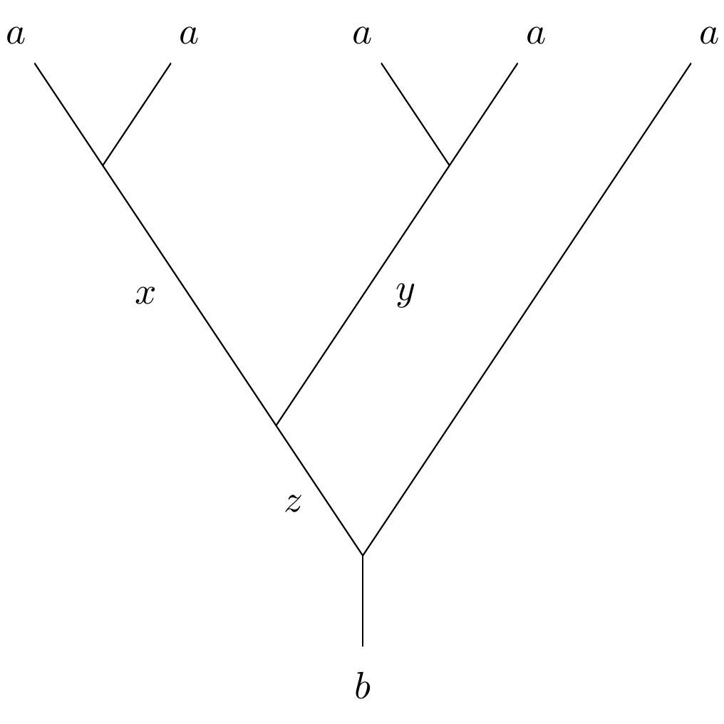

sig is a list of braid group generators as matrices. In some cases these will be represented as sparse matrices.

In the following example we compute a 5-dimensional braid group representation on 5 strands associated to the spin representation in the modular tensor category \(SU(2)_4 \cong SO(3)_2\).

EXAMPLES:

Sage

sage: A14 = FusionRing("A1", 4)
sage: A14.get_order()
[(0, 0), (1/2, -1/2), (1, -1), (3/2, -3/2), (2, -2)]
sage: A14.fusion_labels(["one", "two", "three", "four", "five"], inject_variables=True)
sage: [A14(x) for x in A14.get_order()]
[one, two, three, four, five]
sage: two ** 5
5*two + 4*four
sage: comp_basis, sig = A14.get_braid_generators(two, two, 5, verbose=False) # long time
sage: A14.gens_satisfy_braid_gp_rels(sig)                                 # long time
True
sage: len(comp_basis) == 5                                                # long time
True

Python

>>> from sage.all import *
>>> A14 = FusionRing("A1", Integer(4))
>>> A14.get_order()
[(0, 0), (1/2, -1/2), (1, -1), (3/2, -3/2), (2, -2)]
>>> A14.fusion_labels(["one", "two", "three", "four", "five"], inject_variables=True)
>>> [A14(x) for x in A14.get_order()]
[one, two, three, four, five]
>>> two ** Integer(5)
5*two + 4*four
>>> comp_basis, sig = A14.get_braid_generators(two, two, Integer(5), verbose=False) # long time
>>> A14.gens_satisfy_braid_gp_rels(sig)                                 # long time
True
>>> len(comp_basis) == Integer(5)                                                # long time
True

get_computational_basis(a, b, n_strands)

Return the so-called computational basis for \(\text{Hom}(b, a^n)\).

INPUT:

• a – a basis element

• b – another basis element

• n_strands – the number of strands for a braid group

Let \(n=\) n_strands and let \(k\) be the greatest integer \(\leq n/2\). The braid group acts on \(\text{Hom}(b, a^n)\). This action is computed in get_braid_generators(). This method returns the computational basis in the form of a list of fusion trees. Each tree is represented by an \((n-2)\)-tuple

\[(m_1, \ldots, m_k, l_1, \ldots, l_{k-2})\]

such that each \(m_j\) is an irreducible constituent in \(a \otimes a\) and

\[\begin{split}\begin{array}{l} b \in l_{k-2} \otimes m_{k}, \\ l_{k-2} \in l_{k-3} \otimes m_{k-1}, \\ \cdots, \\ l_2 \in l_1 \otimes m_3, \\ l_1 \in m_1 \otimes m_2, \end{array}\end{split}\]

where \(z \in x \otimes y\) means \(N_{xy}^z \neq 0\).

As a computational device when n_strands is odd, we pad the vector \((m_1, \ldots, m_k)\) with an additional \(m_{k+1}\) equal to \(a\). However, this \(m_{k+1}\) does not appear in the output of this method.

The following example appears in Section 3.1 of [CW2015].

EXAMPLES:

Sage

sage: A14 = FusionRing("A1", 4)
sage: A14.get_order()
[(0, 0), (1/2, -1/2), (1, -1), (3/2, -3/2), (2, -2)]
sage: A14.fusion_labels(["zero", "one", "two", "three", "four"], inject_variables=True)
sage: [A14(x) for x in A14.get_order()]
[zero, one, two, three, four]
sage: A14.get_computational_basis(one, two, 4)
[(two, two), (two, zero), (zero, two)]

Python

>>> from sage.all import *
>>> A14 = FusionRing("A1", Integer(4))
>>> A14.get_order()
[(0, 0), (1/2, -1/2), (1, -1), (3/2, -3/2), (2, -2)]
>>> A14.fusion_labels(["zero", "one", "two", "three", "four"], inject_variables=True)
>>> [A14(x) for x in A14.get_order()]
[zero, one, two, three, four]
>>> A14.get_computational_basis(one, two, Integer(4))
[(two, two), (two, zero), (zero, two)]

get_fmatrix(*args, **kwargs)

Construct an FMatrix factory to solve the pentagon relations and organize the resulting F-symbols.

EXAMPLES:

Sage

sage: A15 = FusionRing("A1", 5)
sage: A15.get_fmatrix()
F-Matrix factory for The Fusion Ring of Type A1 and level 5 with Integer Ring coefficients

Python

>>> from sage.all import *
>>> A15 = FusionRing("A1", Integer(5))
>>> A15.get_fmatrix()
F-Matrix factory for The Fusion Ring of Type A1 and level 5 with Integer Ring coefficients

get_order()

Return the weights of the basis vectors in a fixed order.

You may change the order of the basis using CombinatorialFreeModule.set_order()

EXAMPLES:

Sage

sage: A15 = FusionRing("A1", 5)
sage: w = A15.get_order(); w
[(0, 0), (1/2, -1/2), (1, -1), (3/2, -3/2), (2, -2), (5/2, -5/2)]
sage: A15.set_order([w[k] for k in [0, 4, 1, 3, 5, 2]])
sage: [A15(x) for x in A15.get_order()]
[A15(0), A15(4), A15(1), A15(3), A15(5), A15(2)]

Python

>>> from sage.all import *
>>> A15 = FusionRing("A1", Integer(5))
>>> w = A15.get_order(); w
[(0, 0), (1/2, -1/2), (1, -1), (3/2, -3/2), (2, -2), (5/2, -5/2)]
>>> A15.set_order([w[k] for k in [Integer(0), Integer(4), Integer(1), Integer(3), Integer(5), Integer(2)]])
>>> [A15(x) for x in A15.get_order()]
[A15(0), A15(4), A15(1), A15(3), A15(5), A15(2)]

Warning

This duplicates get_order() from CombinatorialFreeModule except the result is not cached. Caching of CombinatorialFreeModule.get_order() causes inconsistent results after calling CombinatorialFreeModule.set_order().

global_q_dimension(base_coercion=True)

Return \(\sum d_i^2\), where the sum is over all simple objects and \(d_i\) is the quantum dimension.

The global \(q\)-dimension is a positive real number.

EXAMPLES:

Sage

sage: FusionRing("E6", 1).global_q_dimension()
3

Python

>>> from sage.all import *
>>> FusionRing("E6", Integer(1)).global_q_dimension()
3

is_multiplicity_free()

Return True if the fusion multiplicities Nk_ij() are bounded by 1.

The FMatrix is available only for multiplicity free instances of FusionRing.

EXAMPLES:

Sage

sage: [FusionRing(ct, k).is_multiplicity_free() for ct in ("A1", "A2", "B2", "C3") for k in (1, 2, 3)]
[True, True, True, True, True, False, True, True, False, True, False, False]

Python

>>> from sage.all import *
>>> [FusionRing(ct, k).is_multiplicity_free() for ct in ("A1", "A2", "B2", "C3") for k in (Integer(1), Integer(2), Integer(3))]
[True, True, True, True, True, False, True, True, False, True, False, False]

r_matrix(i, j, k, base_coercion=True)

Return the R-matrix entry corresponding to the subobject k in the tensor product of i with j.

Warning

This method only gives complete information when \(N_{ij}^k = 1\) (an important special case). Tables of MTC including R-matrices may be found in Section 5.3 of [RoStWa2009] and in [Bond2007].

The R-matrix is a homomorphism \(i \otimes j \rightarrow j \otimes i\). This may be hard to describe since the object \(i \otimes j\) may be reducible. However if \(k\) is a simple subobject of \(i \otimes j\) it is also a subobject of \(j \otimes i\). If we fix embeddings \(k \rightarrow i \otimes j\), \(k \rightarrow j \otimes i\) we may ask for the scalar automorphism of \(k\) induced by the R-matrix. This method computes that scalar. It is possible to adjust the set of embeddings \(k \rightarrow i \otimes j\) (called a gauge) so that this scalar equals

\[\pm \sqrt{\frac{ \theta_k }{ \theta_i \theta_j }}.\]

If \(i \neq j\), the gauge may be used to control the sign of the square root. But if \(i = j\) then we must be careful about the sign. These cases are computed by a formula of [BDGRTW2019], Proposition 2.3.

EXAMPLES:

Sage

sage: I = FusionRing("E8", 2, conjugate=True)  # Ising MTC
sage: I.fusion_labels(["i0", "p", "s"], inject_variables=True)
sage: I.r_matrix(s, s, i0) == I.root_of_unity(-1/8)
True
sage: I.r_matrix(p, p, i0)
-1
sage: I.r_matrix(p, s, s) == I.root_of_unity(-1/2)
True
sage: I.r_matrix(s, p, s) == I.root_of_unity(-1/2)
True
sage: I.r_matrix(s, s, p) == I.root_of_unity(3/8)
True

Python

>>> from sage.all import *
>>> I = FusionRing("E8", Integer(2), conjugate=True)  # Ising MTC
>>> I.fusion_labels(["i0", "p", "s"], inject_variables=True)
>>> I.r_matrix(s, s, i0) == I.root_of_unity(-Integer(1)/Integer(8))
True
>>> I.r_matrix(p, p, i0)
-1
>>> I.r_matrix(p, s, s) == I.root_of_unity(-Integer(1)/Integer(2))
True
>>> I.r_matrix(s, p, s) == I.root_of_unity(-Integer(1)/Integer(2))
True
>>> I.r_matrix(s, s, p) == I.root_of_unity(Integer(3)/Integer(8))
True

root_of_unity(r, base_coercion=True)

Return \(e^{i\pi r}\) as an element of self.field() if possible.

INPUT:

• r – a rational number

EXAMPLES:

Sage

sage: A11 = FusionRing("A1", 1)
sage: A11.field()
Cyclotomic Field of order 24 and degree 8
sage: for n in [1..7]:
....:     try:
....:         print(n, A11.root_of_unity(2/n))
....:     except ValueError as err:
....:         print(n, err)
1 1
2 -1
3 zeta24^4 - 1
4 zeta24^6
5 not a root of unity in the field
6 zeta24^4
7 not a root of unity in the field

Python

>>> from sage.all import *
>>> A11 = FusionRing("A1", Integer(1))
>>> A11.field()
Cyclotomic Field of order 24 and degree 8
>>> for n in (ellipsis_range(Integer(1),Ellipsis,Integer(7))):
...     try:
...         print(n, A11.root_of_unity(Integer(2)/n))
...     except ValueError as err:
...         print(n, err)
1 1
2 -1
3 zeta24^4 - 1
4 zeta24^6
5 not a root of unity in the field
6 zeta24^4
7 not a root of unity in the field

s_ij(elt_i, elt_j, base_coercion=True)

Return the element of the \(S\)-matrix of this fusion ring corresponding to the given elements.

This is the unnormalized \(S\)-matrix, denoted \(\tilde{s}_{ij}\) in [BaKi2001] . To obtain the normalized \(S\)-matrix, divide by global_q_dimension() or use S_matrix() with the option unitary=True.

This is computed using the formula

\[s_{i, j} = \frac{1}{\theta_i\theta_j} \sum_k N_{ik}^j d_k \theta_k,\]

where \(\theta_k\) is the twist and \(d_k\) is the quantum dimension. See [Row2006] Equation (2.2) or [EGNO2015] Proposition 8.13.8.

INPUT:

• elt_i, elt_j – elements of the fusion basis

EXAMPLES:

Sage

sage: G21 = FusionRing("G2", 1)
sage: b = G21.basis()
sage: [G21.s_ij(x, y) for x in b for y in b]
[1, -zeta60^14 + zeta60^6 + zeta60^4, -zeta60^14 + zeta60^6 + zeta60^4, -1]

Python

>>> from sage.all import *
>>> G21 = FusionRing("G2", Integer(1))
>>> b = G21.basis()
>>> [G21.s_ij(x, y) for x in b for y in b]
[1, -zeta60^14 + zeta60^6 + zeta60^4, -zeta60^14 + zeta60^6 + zeta60^4, -1]

s_ijconj(elt_i, elt_j, base_coercion=True)

Return the conjugate of the element of the \(S\)-matrix given by self.s_ij(elt_i, elt_j, base_coercion=base_coercion).

See s_ij().

EXAMPLES:

Sage

sage: G21 = FusionRing("G2", 1)
sage: b = G21.basis()
sage: [G21.s_ijconj(x, y) for x in b for y in b]
[1, -zeta60^14 + zeta60^6 + zeta60^4, -zeta60^14 + zeta60^6 + zeta60^4, -1]

Python

>>> from sage.all import *
>>> G21 = FusionRing("G2", Integer(1))
>>> b = G21.basis()
>>> [G21.s_ijconj(x, y) for x in b for y in b]
[1, -zeta60^14 + zeta60^6 + zeta60^4, -zeta60^14 + zeta60^6 + zeta60^4, -1]

This method works with all possible types of fields returned by self.fmats.field().

s_matrix(unitary=False, base_coercion=True)

Return the \(S\)-matrix of this fusion ring.

OPTIONAL:

• unitary – boolean (default: False); set to True to obtain the unitary \(S\)-matrix

Without the unitary parameter, this is the matrix denoted \(\widetilde{s}\) in [BaKi2001].

EXAMPLES:

Sage

sage: D91 = FusionRing("D9", 1)
sage: D91.s_matrix()
[          1           1           1           1]
[          1           1          -1          -1]
[          1          -1 -zeta136^34  zeta136^34]
[          1          -1  zeta136^34 -zeta136^34]
sage: S = D91.s_matrix(unitary=True); S
[            1/2             1/2             1/2             1/2]
[            1/2             1/2            -1/2            -1/2]
[            1/2            -1/2 -1/2*zeta136^34  1/2*zeta136^34]
[            1/2            -1/2  1/2*zeta136^34 -1/2*zeta136^34]
sage: S*S.conjugate()
[1 0 0 0]
[0 1 0 0]
[0 0 1 0]
[0 0 0 1]

Python

>>> from sage.all import *
>>> D91 = FusionRing("D9", Integer(1))
>>> D91.s_matrix()
[          1           1           1           1]
[          1           1          -1          -1]
[          1          -1 -zeta136^34  zeta136^34]
[          1          -1  zeta136^34 -zeta136^34]
>>> S = D91.s_matrix(unitary=True); S
[            1/2             1/2             1/2             1/2]
[            1/2             1/2            -1/2            -1/2]
[            1/2            -1/2 -1/2*zeta136^34  1/2*zeta136^34]
[            1/2            -1/2  1/2*zeta136^34 -1/2*zeta136^34]
>>> S*S.conjugate()
[1 0 0 0]
[0 1 0 0]
[0 0 1 0]
[0 0 0 1]

some_elements()

Return some elements of self.

EXAMPLES:

Sage

sage: D41 = FusionRing('D4', 1)
sage: D41.some_elements()
[D41(1,0,0,0), D41(0,0,1,0), D41(0,0,0,1)]

Python

>>> from sage.all import *
>>> D41 = FusionRing('D4', Integer(1))
>>> D41.some_elements()
[D41(1,0,0,0), D41(0,0,1,0), D41(0,0,0,1)]

test_braid_representation(max_strands=6, anyon=None)

Check that we can compute valid braid group representations.

INPUT:

• max_strands – (default: 6) maximum number of braid group strands

• anyon – (optional) run this test on this particular simple object

Create a braid group representation using get_braid_generators() and confirms the braid relations. This test indirectly partially verifies the correctness of the orthogonal F-matrix solver. If the code were incorrect the method would not be deterministic because the fusing anyon is chosen randomly. (A different choice is made for each number of strands tested.) However the doctest is deterministic since it will always return True. If the anyon parameter is omitted, a random anyon is tested for each number of strands up to max_strands.

EXAMPLES:

Sage

sage: A21 = FusionRing("A2", 1)
sage: A21.test_braid_representation(max_strands=4)
True
sage: F41 = FusionRing("F4", 1)            # long time
sage: F41.test_braid_representation()      # long time
True

Python

>>> from sage.all import *
>>> A21 = FusionRing("A2", Integer(1))
>>> A21.test_braid_representation(max_strands=Integer(4))
True
>>> F41 = FusionRing("F4", Integer(1))            # long time
>>> F41.test_braid_representation()      # long time
True

total_q_order(base_coercion=True)

Return the positive square root of self.global_q_dimension() as an element of self.field().

This is implemented as \(D_{+}e^{-i\pi c/4}\), where \(D_+\) is D_plus() and \(c\) is virasoro_central_charge().

EXAMPLES:

Sage

sage: F = FusionRing("G2", 1)
sage: tqo=F.total_q_order(); tqo
zeta60^15 - zeta60^11 - zeta60^9 + 2*zeta60^3 + zeta60
sage: tqo.is_real_positive()
True
sage: tqo^2 == F.global_q_dimension()
True

Python

>>> from sage.all import *
>>> F = FusionRing("G2", Integer(1))
>>> tqo=F.total_q_order(); tqo
zeta60^15 - zeta60^11 - zeta60^9 + 2*zeta60^3 + zeta60
>>> tqo.is_real_positive()
True
>>> tqo**Integer(2) == F.global_q_dimension()
True

twists_matrix()

Return a diagonal matrix describing the twist corresponding to each simple object in the FusionRing.

EXAMPLES:

Sage

sage: B21=FusionRing("B2", 1)
sage: [x.twist() for x in B21.basis().list()]
[0, 1, 5/8]
sage: [B21.root_of_unity(x.twist()) for x in B21.basis().list()]
[1, -1, zeta32^10]
sage: B21.twists_matrix()
[        1         0         0]
[        0        -1         0]
[        0         0 zeta32^10]

Python

>>> from sage.all import *
>>> B21=FusionRing("B2", Integer(1))
>>> [x.twist() for x in B21.basis().list()]
[0, 1, 5/8]
>>> [B21.root_of_unity(x.twist()) for x in B21.basis().list()]
[1, -1, zeta32^10]
>>> B21.twists_matrix()
[        1         0         0]
[        0        -1         0]
[        0         0 zeta32^10]

virasoro_central_charge()

Return the Virasoro central charge of the WZW conformal field theory associated with the Fusion Ring.

If \(\mathfrak{g}\) is the corresponding semisimple Lie algebra, this is

\[\frac{k\dim\mathfrak{g}}{k+h^\vee},\]

where \(k\) is the level and \(h^\vee\) is the dual Coxeter number. See [DFMS1996] Equation (15.61).

Let \(d_i\) and \(\theta_i\) be the quantum dimensions and twists of the simple objects. By Proposition 2.3 in [RoStWa2009], there exists a rational number \(c\) such that \(D_+ / \sqrt{D} = e^{i\pi c/4}\), where \(D_+ = \sum d_i^2 \theta_i\) is computed in D_plus() and \(D = \sum d_i^2 > 0\) is computed by global_q_dimension(). Squaring this identity and remembering that \(D_+ D_- = D\) gives

\[D_+ / D_- = e^{i\pi c/2}.\]

EXAMPLES:

Sage

sage: R = FusionRing("A1", 2)
sage: c = R.virasoro_central_charge(); c
3/2
sage: Dp = R.D_plus(); Dp
2*zeta32^6
sage: Dm = R.D_minus(); Dm
-2*zeta32^10
sage: Dp / Dm == R.root_of_unity(c/2)
True

Python

>>> from sage.all import *
>>> R = FusionRing("A1", Integer(2))
>>> c = R.virasoro_central_charge(); c
3/2
>>> Dp = R.D_plus(); Dp
2*zeta32^6
>>> Dm = R.D_minus(); Dm
-2*zeta32^10
>>> Dp / Dm == R.root_of_unity(c/Integer(2))
True